Analysis of Dynamic Voltage Scaling for System Level Energy ManagementGaurav Dhiman (Department of CSE, UC San Diego) Kishore Kumar Pusukuri (Department of CSE, UC Riverside) Tajana Rosing (Department of CSE, UC San Diego) |
Abstract: In this paper we show that in modern computing systems, DVFS gives much more limited energy savings with relatively high performance overhead as compared to running workloads at high speed and then transitioning into low power state. The primary reasons for this are recent advancements in platform and CPU architectures such as sophisticated memory subsystem design, and more efficient low power state support. We justify our analysis with measurements on a state of the art system using benchmarks ranging from very CPU intensive to memory intensive workloads.
Power consumption has become an over-riding concern in the design of computer systems today. Dynamic voltage frequency scaling (DVFS) is a power management technique, that dynamically scales the voltage and frequency (v-f) settings of the CPU so as to provide “just-enough” speed to process the system workload. Scaling down of voltage levels results in a quadratic reduction in CPUs dynamic power consumption. Many modern CPUs such as AMD Opteron and Intel Xeon are equipped with DVFS capability [1].
Previous work (explained in section 2) on DVFS has reported results that demonstrate its ability to achieve energy savings while keeping the performance degradation under acceptable limits. Though the basic ideas in these policies are scalable across architectures, it is difficult to understand how the energy savings and performance change due to newer technologies and system design. For instance, policies proposed in [2] and [3] assume that it is always beneficial to minimize the CPU idle periods by scaling down the frequency. This assumption was true when these policies were designed, since the idle CPU used to consume a lot of power. However, it is no longer the case, since recent processors have introduced efficient support for low power modes that can reduce the power consumption to near zero. This changes the applicability of such policies for current generation of processors. In addition, the increasing power consumption of other system components like memory can significantly change the possible benefits of DVFS. Hence, it is important to understand the benefits of DVFS from the whole system standpoint.
In this work we show experimentally and through analysis that the potential for energy savings with DVFS has significantly diminished in newer CPU technologies due to faster memory interface system, more efficient support for low power modes in CPUs and higher relative power consumption of components other than CPU (e.g. memory). We further provide a key insight that simple power management policies based on low power states of system components provide better system energy savings/performance tradeoffs across a wide range of workloads than DVFS.
The rest of the paper is organized as follows. We discuss the related work in section 2 followed by the background on DVFS and the motivation for our work in section 3. In section 4 we provide an overview of our evaluation setup and elaborate on our experiments and results before finally concluding in section 5.
Previous DVFS-related work may be broadly divided into three categories. The first category of techniques target real time systems, where the task arrival times, workload and deadlines are known in advance [4, 5]. The second category of techniques require either application or compiler support for performing DVFS [6, 7]. The third category comprises of system level DVFS techniques that do not rely on any application/compiler level support and target general purpose systems. The work done in [2, 3] monitor CPU utilization at regular intervals and performs dynamic scaling based on their estimate of utilization for the next interval. The premise is to shorten the idle period as much as possible using scaling, since it is always beneficial to do so from energy savings perspective. As we show in our work, this assumption is no longer true. The work done in [8, 9] characterize the running tasks and accordingly make the voltage scaling decisions only for those phases of the tasks where it is beneficial. Further, the policies take DVFS decisions based on how beneficial they are from CPU energy savings perspective. We show that doing so does not necessarily result in higher system level energy savings as well. In contrast, we show that simple power management policies based on utilizing the low power modes commonly available in modern processors and memories can provide better energy savings and performance tradeoffs.
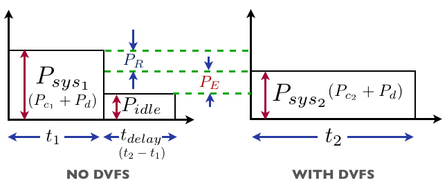
Figure 1: Power Consumption and Execution Times
Figure 1 illustrates system power consumption with and without DVFS for a workload. Without DVFS the CPU executes the workload at the highest frequency for time t1 and the system consumes power Psys1. When not executing anything useful, the system/CPU is idle and consumes power Pidle. With DVFS the power consumption reduces to Psys2, while the execution time increases by tdelay from t1 to t1+tdelay (shown as t2) because of CPU operation at a lower v-f setting. The decrease in power consumption depends on the degree of reduction in voltage and frequency, while the increase in execution time of the workload (tdelay) is a function of how it utilizes the CPU resources [8, 9]. We can further break down the system power consumption into that of CPU (Pc) and the other devices in the system (Pd). If we let the power consumption of CPU at v-f settings 1 and 2 by Pc1 and Pc2 respectively, and Pcidle, when it is idle (as shown in Figure 1), we can represent the energy savings due to DVFS as:
PR/ER is the reduction in CPU power/energy consumption because of DVFS. The second term (PEtdelay/EE) represents the extra energy consumption that DVFS causes relative to the case without DVFS. There are two sources of extra power consumption for a system with DVFS: 1) The difference between CPU power consumption at the lower v-f setting and the idle CPU (Pc2 − Pcidle), 2) The difference between device power consumption when it is active and idle (Pd − Pdidle). The extra device power consumption depends on how often the executing workload accesses the devices. For instance, for a memory bound workload, the difference would be high, since it would make the memory consume more power for the extra time tdelay compared to an idle system. In contrast, for a CPU bound workload, the difference would be negligible. The performance delay (tdelay) determines for how long the DVFS based system consumes this additional power, and hence the extra energy consumption (EE).
Clearly, the DVFS provides energy savings only as long as ER > EE. When this inequality does not hold, the system incurs performance overhead (tdelay) and consumes more energy than when running at the highest CPU frequency. We next show how the performance delay, low overhead of entry into sleep states and the energy impact of other system components affects the efficiency of DVFS.
A memory bound workload incurs lower performance hit at a lower frequency setting, since it causes many CPU stalls due to memory accesses [8, 9]. For an ideal stall intensive workload, the delay in execution is zero, and hence represents the best case for DVFS. In contrast, the execution time of a CPU intensive workload is entirely determined by the CPU frequency. For an ideal CPU intensive workload, the increase in execution time when switching from frequency f1 to f2 can be estimated as (f1/f2). Such a workload represents the worst case for DVFS, since it incurs the highest possible tdelay.
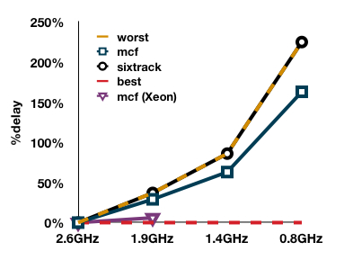
In SPECCPU 2000 suite, mcf is the most memory bound benchmark, while sixtrack is one of the most CPU intensive [10]. To understand the correlation between execution time delay and workload characteristics we ran the benchmarks at different frequency settings on a state of the art quad core AMD Opteron based OpenSolaris system. Table 2 shows the %delay incurred by the benchmarks at the four settings supported by the processor. We also plot the %delay for an ideal CPU intensive workload, which we label as the“worst” case, and for the ideal stall intensive workload, which we label as the “best” case. Sixtrack incurs a delay that is identical to that of the worst case due to its high CPU intensiveness. In contrast, for mcf it is relatively lower.
However, this delay is significantly larger than the best case. This delay is much smaller on processors with smaller caches and slower memory controllers. The AMD processor we use has three levels of caches (L3 cache of 6MB), an on-die memory controller that operates at 2.6GHz and sophisticated cache prefetching mechanisms. Consequently, the memory bound phases of mcf are much shorter on this processor compared to running it on a processor with slower memory accesses. For instance, running mcf on an older Intel quad core Xeon (with two frequency settings: 2.6/1.9GHz, no L3 cache and an off chip memory controller), the delay of mcf at 1.9GHz is just 6% from the best case (see Figure 2). This is much lower when compared to 30% delay on the Opteron at the same frequency. Faster memory controllers and larger caches successfully mask the memory latency making the execution more dependent on the CPU frequency, thus limiting the possible energy savings due to DVFS.
The support for ACPI C-states or CPU low power states/modes has evolved significantly over the last few years. The C1 state, where the clock supply to the CPU is gated, is so efficient in modern processors, that it is currently used by default in all major operating systems (eg. Linux, OpenSolaris) when CPU is idle. Recently announced Intel and AMD processors have also added support for deeper C states which can signifcantly reduce the power consumption of CPU during idle times [11]. For instance, C6 power state can reduce the power consumption to zero. The roundtrip overhead of such states is in the order of just µ-seconds, thus allowing their frequent use. The previous generation processors did not have such C-state support, and thus consumed higher power during the idle periods. But newer CPUs, that are equipped with these states, can use them effectively to decrease their idle time power consumption. This increases the difference between the CPU power consumption at lower v-f setting and idle time, or in terms of equation 1, increases (Pc2 − Pcidle), and hence EE (see Figure 1).
An important aspect that is often ignored by research in DVFS is its impact on system level power savings. This is important to consider since workloads can make other system components consume more power for a longer duration due to DVFS. For instance, our Opteron system is equipped with 4GB DDR3 RAM, which approximately consumes 4.5W when it is idle/not being accessed. However, when a memory intensive benchmark (like mcf) is running, the memory consumption increases by 5W, i.e. it more than doubles. Thus, running mcf at a lower frequency makes the memory consume extra 5W for tdelay (see Figure 1), compared to a system without DVFS. This means a higher value of (Pd − Pdidle), or higher EE (see Figure 1).
Policy name Description PM-1 switch CPU to ACPI state C1 (remove clock supply) and move to lowest voltage setting PM-2 switch CPU to ACPI state C6 (remove power) PM-3 switch CPU to ACPI state C6 and switch the memory to self-refresh mode
Table 1: Power Management Policies
To evaluate the effectiveness of DVFS for system level energy savings we formulate a simple static DVFS policy (s-DVFS), where workloads are executed statically at different v-f settings. This is sub-optimal, since one can potentially get better results by running a workload at different settings based on its phase of execution. However, as we show later, it does give a fair idea of the possible savings in the best case for most of the benchmarks. We also propose three simple power management policies that are based on running the workload at the highest speed and then reducing the power during the idle periods (Pidle in Figure 1) through different mechanisms. These policies are listed in Table 1. Each policy is successively more aggressive than the previous one in terms of reducing Pidle. PM-1 is extremely easy to implement as support for C1 states is widely available in current processors. PM-2 relies on efficient C6 state support, which has recently been introduced in Intel and AMD processors. PM-3 is the most aggressive as it puts the memory into self-refresh mode thereby getting higher system level savings. We assume availability of low overhead entry/exit from self-refresh mode. The motivation of our evaluation is to compare the performance of s-DVFS against these three policies.
For our experiments, we instrument a quad core AMD Opteron processor based system running OpenSolaris. The processor supports four v-f settings: 1.25V/2.6GHz, 1.15V/1.9GHz, 1.05V/1.4GHz and 0.9V/0.8GHz. For workloads, we use integer and floating point benchmarks from the SPECCPU 2000 suite. For comparison of s-DVFS with the other PM policies in Table 1, we use the model developed in section 3 (see equation 1). For instance to compare s-DVFS and PM-1, we run the benchmarks at all the frequencies and measure the corresponding execution time and system power. In terms of Figure 1, we get t1 and Psys1, i.e. time and power for the highest frequency (we use that for PM-1) and t2 and Psys2 for the lower frequencies(we use that for s-DFVS). We measure power at the power outlet of the system using a data acquisition system (DAQ), which collects power samples every 300ms. These measurements allow us to estimate PR, PE, t1 and tdelay (see Figure 1), and hence EDVFS based on equation 1 for each frequency ’f’. In other words EDVFS gives the energy savings of s-DVFS over PM-1. Based on this, we estimate the %energy savings of s-DVFS over PM-1 at given frequency ’f’ as:
|
EPM−i varies based on the policy we are comparing s-DVFS against, since each has different idle system power consumption or Pidle (see Table 1). We measure the CPU and memory power consumption separately to estimate Pidle for PM-(1-3).
Table 2 shows the comparison of energy and performance results achieved for s-DVFS and policies PM-(1-3) across 18 SPEC benchmarks. The "frequency" column indicates the frequency (in GHz) at which the processor is set for s-DVFS policy. The %delay indicates the percentage by which the benchmark’s execution time increases because of s-DVFS when compared against policies PM-(1-3). The %energy savings (%EsavingsPM−i) column indicates the system level energy savings achieved by the s-DVFS policy compared to the PM-(1-3) based on equation 2. Positive savings indicate that s-DVFS at the given frequency is more energy efficient than the corresponding PM policy and vice versa.
SPEC 2000 INT
Table 2: Comparison of s-DVFS and PM 1-3
Workload freq %delay %EsavingsPM−i PM-1 PM-2 PM-3 mcf 1.9 29% 5.2% 0.7% -0.5% 1.4 63% 8.1% 0.1% -2.1% 0.8 163% 8.1% -6.3% -10.7% bzip2 1.9 37.1% 4.7% -0.6% -2.0% 1.4 85.7% 7.4% -2.4% -5.2% 0.8 222.9% 7.8% -9.0% -14.2% eon 1.9 33.3% 4.0% -0.9% -2.3% 1.4 81.0% 6.6% -3.1% -5.8% 0.8 219.0% 7.1% -9.9% -15.1% crafty 1.9 37.6% 4.7% -0.6% -2.1% 1.4 85.5% 7.5% -2.3% -5.1% 0.8 222.4% 7.9% -8.9% -14.1% gcc 1.9 34.7% 4.3% -0.7% -2.0% 1.4 81.3% 7.4% -2.0% -4.6% 0.8 214.2% 7.9% -8.6% -13.7% gzip 1.9 36.6% 6.4% 1.3% -0.1% 1.4 85.2% 8.4% -1.2% -4.0% 0.8 224.7% 7.9% -8.9% -14.1% parser 1.9 35.8% 4.4% -0.9% -2.3% 1.4 82.1% 7.0% -2.7% -5.5% 0.8 214.8% 8.0% -8.6% -13.8% twolf 1.9 35.1% 4.5% -0.8% -2.2% 1.4 80.5% 6.8% -2.8% -5.6% 0.8 211.4% 7.1% -9.6% -14.8% vortex 1.9 34.2% 6.8% 2.0% 0.05% 1.4 80.5% 7.5% -1.8% -4.5% 0.8 205.3% 8.2% -7.9% -12.9% vpr 1.9 35.5% 2.7% -2.7% -4.1% 1.4 82.1% 7.1% -2.5% -5.3% 0.8 216.4% 7.6% -9.2% -14.4%
SPEC 2000 FP
Workload freq %delay %EsavingsPM−i PM-1 PM-2 PM-3 sixtrack 1.9 37.3% 5.0% -0.5% -2.0% 1.4 86.2% 6.0% -4.3% -7.2% 0.8 226.4% 6.8% -10.7% -16.1% mesa 1.9 36.5% 2.9% -2.5% -4.0% 1.4 84.8% 5.8% -4.2% -7.0% 0.8 223.8% 7.2% -9.9% -15.2% lucas 1.9 29% 4.3% 0.2% -0.9% 1.4 63.2% 6.7% -1.0% -3.1% 0.8 169.4% 6.1% -8.5% -12.9% swim 1.9 31.8% 3.3% -1.2% -2.4% 1.4 75.2% 3.9% -5.0% -7.4% 0.8 198.4% 4.2% -11.9% -16.8% art 1.9 32.4% 5.9% 1.2% -0.01% 1.4 76.1% 7.3% -1.7% -4.2% 0.8 202.4% 8.0% -8.0% -12.9% mgrid 1.9 31.1% 2.9% -1.6% -2.8% 1.4 79.2% 4.1% -5.3% -7.9% 0.8 208.5% 4.3% -12.3% -17.4% ammp 1.9 35.6% 5.0% -0.2% -1.7% 1.4 83.3% 6.6% -3.3% -6.1% 0.8 218.8% 2.0% -16.0% -21.6% applu 1.9 32.5% 2.7% -2.1% -3.4% 1.4 73.9% 4.7% -4.4% -6.9% 0.8 193.9% 5.7% -10.3% -15.2%
We can observe from Table 2 that across all the benchmarks the performance delay because of s-DVFS is large. For 10 benchmarks (bzip2, eon, gcc, crafty, gzip, parser, vpr, sixtrack, mesa, ammp) the performance delay is within 5% of the worst case (refer to Figure 2) due to their high CPU intensiveness. For 6 benchmarks (vortex, art, mgrid, twolf, swim, applu), it is within 15% of the worst case, which means they comprise of some phases of execution, which are memory bound. Only for mcf and lucas it is more than 15%. Thus, in terms of performance all the benchmarks except mcf and lucas take a severe hit because of DVFS. The primary reason for the high delay is the sophisticated memory subsystem of the CPU we use (refer to section 3).
The %energy savings results indicate that s-DVFS is also not very efficient from the perspective of energy savings. Compared to PM-1, it achieves on an average a maximum of just 7% energy savings across all the benchmarks, which comes at the cost of around 208% increase in execution time. We observe two interesting trends in these results: 1) Energy savings has little correlation to benchmark characteristics: This happens due to %delay being uniformly high for most of the benchmarks. Intuitively mcf and lucas should incur higher savings due their lower tdelay. However, as identified in section 3, the memory bound workloads cause the memory to consume extra energy when compared to CPU bound workloads. This offsets their higher CPU energy savings. 2) There is not much gained by running benchmarks at lower v-f settings: Across all the benchmarks, the average gain in energy savings for s-DVFS by switching from 1.9GHz to 0.8GHz is just 2%. For the same switch the increase in performance delay is around 180%. This indicates that the higher power savings at lower v-f setting do not translate into higher energy savings due to higher performance delay at that setting.
In comparison to PM 2 and 3, the results of s-DVFS are worse. Compared to PM-2, for majority of the benchmarks, s-DVFS is actually energy inefficient. The reason for this follows from our analysis on idle CPU power consumption, which is now reduced to zero, in section 3. Consequently, based on equation 1, EE becomes greater than ER. Compared to PM-3, it is even worse, since policy-3 further lowers the idle system power consumption by putting memory into self-refresh mode.
To understand the energy savings under multi-threaded environments, we experimented with multiple instances of SPEC benchmarks. For illustration purposes we have chosen three benchmarks with different characteristics based on %delay results in Table 2: sixtrack, art and mcf. Table 4 shows the %delay and %energy savings results for different combinations of these benchmarks. We can see that for sixtrack there is no change in the %delay results, since being CPU intensive, the threads do not contend with each other for any CPU resources. In case of mcf we observe a bigger drop in %delay, since being memory intensive, the threads contend for the L3 cache. This increases their memory boundedness. For art, the drop is lower because of lesser contention. The drop in %delay for mcf and art results in higher energy savings compared to the single threaded case. For instance, compared to PM-1, the maximum average energy savings for s-DVFS is now 12% (7% in single threaded case). However, that gets reduced to just 6% when compared to PM-3, while still incurring an average delay of 54%. Just like single threaded results, these results also show that the lower v-f settings offer inferior energy performance tradeoffs compared to higher ones.
Table 3: Multi-threaded Results
Workload freq %delay %EsavingsPM−i PM-1 PM-2 PM-3 4-sixtracks 1.9 37.3% 7% 3.2% 2% 1.4 86.2% 11% 3.7% 1.5% 0.8 226.4% 10% -3.8% -8.2% 4-mcfs 1.9 15% 9% 8% 7% 1.4 31% 14% 11% 10% 0.8 90% 13% 5% 3% 4-arts 1.9 20% 9% 7.7% 7% 1.4 56% 13% 8.6% 7.3% 0.8 154% 14% 4.6% 1.7% 2-mcfs+2-six 1.9 20% 10% 8% 7.5% 1.4 44% 13% 8.7% 7.5% 0.8 117% 14% 5% 2.6% 2-arts+2-mcfs 1.9 22% 8% 6% 5.6% 1.4 50% 12% 8% 6.7% 0.8 149% 11% 0.1% -3%
The results indicate that benefits of DVFS from system level energy savings viewpoint has diminished a lot. We draw the following main conclusions from these results: 1) Simple idle power management policies achieve better system level energy performance tradeoffs in majority of the cases. For CPU intensive workloads, DVFS gets negligible energy savings at the cost of large delay. For memory bound workloads, the higher tdelay because of faster memory subsystem and higher extra memory power consumption they cause, has decreased the potential benefits. 2) Lower v-f settings are not beneficial for energy savings. DVFS policies, if used, should employ higher v-f settings, since they get almost equivalent energy savings at much lower delay. 3) On a system with slower memory controllers, and low power system components, DVFS would still get good system level energy savings and performance tradeoff.
In this paper we have provided insights into the effectiveness of DVFS from a system level energy savings perspective. We show through experiments on a modern state of the art system, that a combination of changes in platform and CPU architecture has resulted in diminishing the energy savings potential of DVFS. We show that simple policies based on low power modes of system components can be fairly effective in providing good energy savings and performance compared to DVFS.
This document was translated from LATEX by HEVEA.