LISA '05 Paper
[LISA '05 Technical Program]
Toward a Cost Model for System Administration
Alva L. Couch, Ning Wu, and Hengky Susanto - Tufts
University
Pp. 125-141 of the Proceedings of LISA '05:
Nineteenth Systems Administration Conference,
(San Diego, CA:
USENIX Association, December 2005).
Abstract
The core of system administration is to utilize a set of "best
practices" that minimize cost and result in maximum value, but very
little is known about the true cost of system administration. In this
paper, we define the problem of determining the cost of system
administration. For support organizations with fixed budgets, the
dominant variant cost is the work and value lost due to time spent
waiting for services. We study how to measure and analyze this cost
through a variety of methods, including white-box and black-box
analysis and discrete event simulation. Simple models of cost provide
insight into why some practices cost more than expected, and why
transitioning from one kind of practice to another is costly.
Introduction
What is a set of "best practices"? Ideally, it is a set of
practices that cost the least while having the most value, i.e., a
model of practice for which the ratio value/cost is maximal over the
lifecycle of the equipment being managed. We have not succeeded in
evaluating practices according to this yardstick, however, because
there is no usable model of cost for any particular set of practices.
We would like a model that predicts, based upon particular management
decisions, the total cost of operations that results from those
decisions over the lifecycle of the network being managed. This is one
goal of "analytical or theoretical system administration" [5, 6].
Many system administrators and managers consider a complete cost
model to be an impossible goal for several reasons. First, the actual
cost of system administration is a relatively constant and monolithic
line item in many IT budgets; it is commonly technically infeasible to
break the lump sum cost into component costs for the purpose of
evaluating strategy. Mechanisms for recording day-to-day costs (e.g.,
detailed time sheets) are often more expensive to manage than the
money they might potentially save. And for the organizations whose
audit requirements force them to maintain detailed costing data, these
records are usually confidential and unavailable to researchers
outside the organization. Thus any really usable cost model has to be
practical in not consuming resources, tunable for specific situations
by the end-user, and must allow that user to incorporate confidential
data into the model without divulging it to outsiders.
Currently, instead of considering costs, we justify best practices
by what might best be called a "micro-economic" model. We say that
certain practices "make the job easier", or other weak
justifications. Is "simpler" really "cheaper"? We have yet to
prove this assertion and - in many cases - the microcosmic reasoning
we use today seems to be incorrect at a macrocosmic (lifecycle) scale.
A case in point is the use of automation, which is "better than
manual changes" except that - at a macrocosmic scale - scaling
increases costs in ways that are inconceivable when working on a small
number of machines. The reasons for this apparent contradiction are
deep and will be discussed later in the paper.
Current Ideas About Cost
The first step toward a cost model was made by Patterson [18], who
points out that while "administrative costs" may be fixed and non-varying, the cost of downtime varies with scale of outage and disrupts
more than computer use. Patterson's formula for the cost of downtime
is based upon calculation of two factors we previously ignored as
system administrators: revenue lost and work lost. Even if our system
administration group has a fixed size and operating budget, the cost
of downtime varies with the severity and scope of outage, and
lifecycle cost of operations thus varies with risk of outage.
Patterson also points out that there are more subtle costs to
downtime, including morale and staff attrition. But how do we quantify
these components in a cost model?
Cost modeling also depends upon risk and cost of potential
catastrophes. Apthorpe [1] describes the mathematics of risk modeling
for system administrators. By understanding risk, we can better make
cost decisions; the lifecycle cost of an administrative strategy is
the expected value of cost based upon a risk model, i.e., the sum of
"cost of outcome" times "probability of outcome" over all possible
outcomes.
Cost modeling of risks is not simple; Cowan, et al. [8] point out
that simply and blindly mitigating risks does not lead to a lowest-cost model. It is often better to wait to apply a security patch
rather than applying it when it is posted, because of the likelihood
of downtime resulting from the patch itself. Thus the global minimum
of lifecycle cost is not achieved by simply minimizing perceived
risks; other risks enter the system as a result of mitigating the
perceived ones.
Further, Alva Couch made the bold claim at the last LISA [7] that
the essential barrier to deployment of better configuration management
is "cost of adoption". The reason that configuration management
strategies such as automation are not applied more widely is that it
costs too much to change from unautomated to automated management. But
he stopped short of truly quantifying cost of adoption in that
presentation, due to inadequate models. Meanwhile, many people
pressured him in one way or another to formalize the model and
demonstrate his claims rigorously. This paper is the first small
result of that pressure.
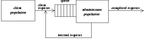
Figure 1: System administration as a queueing
system.
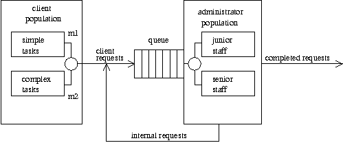
Figure 2: Multiple classes of requests and
administrators.
In this paper, we make the first step toward a cost model for
system administration, based upon related work in other disciplines.
We begin by defining the components of an overall lifecycle cost
model. We look at real data from a trouble-ticketing system to
understand the qualities of load upon a support organization, and
discuss the problems inherent in collecting data from real systems. We
explore the relationship between system administration and capacity
planning, and show that we must determine specific rates in order to
determine costs. We borrow mechanisms for determining those rates from
white-box and black-box cost models in software engineering. Finally,
we turn to discrete event simulation in order to understand the
relationships between rates and cost. As a result, we can begin to
quantify the cost of some decisions about practice, including
deployment schedules for new software.
A Simple Model Of System Administration
First, system administration can be modeled as a queueing system
(Figure 1) in which incoming requests arrive, are queued for later
processing, and eventually dequeued and acted upon, and completed.
Each kind of request arrives at the queue with an "arrival rate" and
is completed in a length of time whose reciprocal represents a
"service rate." We embody all changes made to the network as
requests; a request may indicate a problem or ask for a change in the
nature of services offered. Requests arise from many sources,
including users, management, and even the system administrator herself
may make a note to change something. Likewise, requests are granted
via many mechanisms, including work by system administrators and work
by others.
Note that this is a more complex model than represented by the
typical helpdesk. In a typical ticket system, tickets represent
external requests, while internal requests (e.g.,
actions generated by a security incident report) are not given ticket
numbers. In our request queue, all change actions are entered into the
queue, serviced, and closed when done.
System administration has complex goals, so the request queue has
a complex structure; it is (in the language of capacity planning [17])
a multi-class queueing system consisting of a mixed set of
several "classes" of requests (Figure 2). Many kinds of requests,
with different average arrival rates, are combined into one request
stream. Each kind of request K has a distinct average service rate
 K (and perhaps, a distinct statistical distribution of
service times). As well, a realistic system administration
organization is a non-product system: system administrators do
not function independently like a set of cloned webservers; they
communicate and interact with one another, affecting throughput. A
product system (as in Cartesian product) consists of a number
of components that function independently (so that the state-space of
the whole system is a Cartesian product of the state-spaces of its
parts). K (and perhaps, a distinct statistical distribution of
service times). As well, a realistic system administration
organization is a non-product system: system administrators do
not function independently like a set of cloned webservers; they
communicate and interact with one another, affecting throughput. A
product system (as in Cartesian product) consists of a number
of components that function independently (so that the state-space of
the whole system is a Cartesian product of the state-spaces of its
parts).
Request Arrivals
While the overall structure of the request queue is complex, we
observe that the structure of some classes of requests is easy to
understand. Many classes of requests arrive with a "Poisson
distribution" of inter-arrival times. In a Poisson distribution with
arrival rate of  requests per unit time, requests per unit time,
-
The mean inter-arrival time is 1/.
-
The standard deviation of the inter-arrival time is 1/.
-
The arrival process is memoryless; the probability that a
request will arrive in the next t seconds is independent of whether
one arrived recently.
Many kinds of requests naturally obey this distribution. For
example, any kind of request in which a large population operates
independently of one another has a Poisson distribution, e.g.,
forgotten passwords.
As well, many non-Poisson classes of requests (e.g., virus
attacks) arrive with a Poisson distribution if viewed at the proper
scale. While requests for virus cleaning of individual hosts arrive in
bursts and are not memoryless, the arrival of the virus at one's site
is an independent, memoryless event. If we treat the virus arrival at
one's site as one event, rather than the thousands of requests
it may generate, then new viruses arrive with a roughly Poisson
distribution (because they originate from independent sources at
relatively constant rates). Likewise, while an outage of a
particularly busy server may generate thousands of tickets, the outage
itself obeys a Poisson distribution even though the tickets resulting
from the outage do not. Many other kinds of requests have this
character; although actual tickets arrive in bursts, the real problem
occurs in a memoryless way that is independent of all other problem
occurrences. Examples include hardware failures, power outages,
denial-of-service attacks, spam, etc.
Request Processing
The second part of our model is how requests are processed. Like
request arrivals, request processing is complex but there are parts of
it that are understandable. For example, many kinds of requests are
completed via an "exponential distribution" of service time. The
properties of an exponential service time are similar to those for a
Poisson arrival; if a class of requests is serviced with an
exponential rate of requests per unit time, then:
-
The mean time for servicing a request is 1/.
-
The standard deviation of service time is 1/.
-
The service process is memoryless; the probability that a
request will be finished in the next t seconds is independent of
whether we know it has been in progress for s seconds already.
The last assumption might be paraphrased "A watched pot never
boils."
Examples of requests that exhibit an exponential service time
include password resets, routine account problems, server crashes,
etc. For each of these, there is a rate of response that is
independent of the nature of the specific request (i.e., which user)
and seldom varies from a given average rate . Requests that cannot
be serviced via an exponential distribution include complex
troubleshooting tasks, and any request where the exact method of
solution is unknown at the time of request. In general, a request for
which the answer is well documented and scripted exhibits an
exponential distribution of service times; requests with no documented
response do not.
Lessons From Capacity Planning
Real data discussed below shows that inter-arrival times may
not exhibit a Poisson distribution, and that service times may not
be exponentially distributed. However, much is known about the
performance of idealized queues governed by Poisson and exponential
distributions, and there are many system administration tasks for
which these performance estimates are reasonable.
A queue that exhibits Poisson arrivals with rate and has c independent system
administrators working with service rates
is called an "M/M/c" queue. The first M stands for
`memoryless' (Poisson) arrivals, the second M stands for `memoryless'
(exponential) service times, and c is a count of servers
(administrators) all of whom complete requests with rate . The behavior of an M/M/c queue is
well understood and is commonly used for capacity planning of server
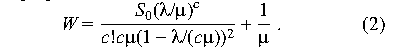
farms and IT infrastructure. For an M/M/c queue, whenever
/c
< 1, the probability that the queue is empty is
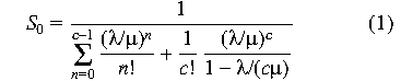 and the "mean time in system" (average wait) for a request [15] is
The mean time spent waiting for n requests to be serviced is n
times the mean wait for one. More important, this equation allows us
to predict whether adding more system administrators will not solve a
response-time problem. As c grows, the first term of the above
equation goes to 0 and the response time converges toward the
theoretical minimum 1/.
Many other equations and relationships exist for more general
queues. In this paper, we will consider only M/M/c models; for an
excellent guide to other models and how to predict performance from
them (including excel spreadsheets for decision support), see [17].
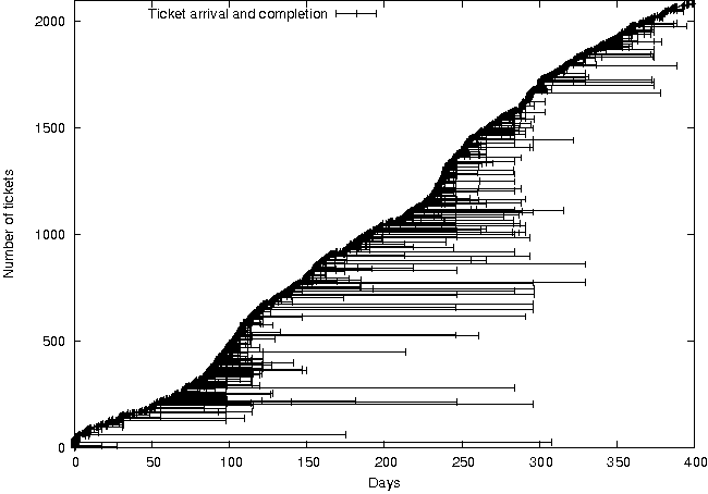
Figure 3: Ticket durations in ECE/CS from 7/2004 to
7/2005.
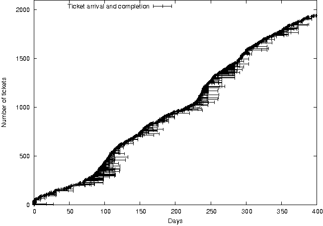
Figure 4: Ticket durations less than 30
days.
Learning From Real Data
From above, it is easy to analyze systems that behave according to
Poisson arrivals and exponential service. How realistic are these
assumptions about system administration? To explore this, we examined
a ticket queue from a live site (Tufts ECE/CS). Note that no one knew,
until very recently, that anyone was going to analyze this ticket
data. It is thus free of many sampling biases. It is, however,
difficult to determine exactly when many tickets were closed. This is
because there is no site requirement to close tickets promptly, and
many tickets are closed by student staff who monitor the ticket queue,
sometimes long after the problem has been addressed.
Plotting ticket numbers (an increasing sequence) against time
(Figure 3) shows little or no evocative patterns. Each ticket is
plotted as a horizontal line, with beginning and end representing
creation and completion time. The Y axis represents ticket number;
tickets due to spam have been deleted and the resulting queue
renumbered as increasing integers with no gaps. Note particularly that
several tickets are still open after several months.
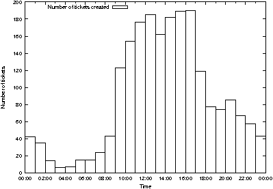
Figure 5: Ticket arrivals exhibit sinusoidal rate
variation over 24 hours.
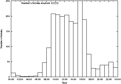
Figure 6: Ticket closures exhibit a sinusoidal time
distribution with a hotspot at 15:00-16:00.
We discovered very quickly that there were two classes of service:
one for short-duration requests and another for long-duration
requests. Viewed alone, the requests that took less than a month
exhibit relatively consistent response times (Figure 4).
Request arrivals are not Poisson. For arrivals to exhibit a
Poisson distribution, the mean of inter-arrival times must be equal to
their standard deviation. In this case, the overall standard deviation
of inter-arrival times (9580 seconds or  2.65 hours) is about
1.37 times the mean (6971 seconds or 1.94 hours), indicating
that there are periods of inactivity. Looking deeper, Figure 5 shows
one problem: arrival rates are not constant, but instead sinusoidal
over a 24-hour period. In this graph, ticket arrivals are shown by
hour, summed over the lifetime of the Request Tracker (RT) database.
The times are corrected for daylight savings time, and show more
intense traffic 9 am to 5 pm with a small dip in traffic at lunch.
Ticket closures show a different pattern (Figure 6) with a hotspot at
3 pm that defies explanation, until one realizes that a student
administrator charged with monitoring and closing tickets starts work
at that time! 2.65 hours) is about
1.37 times the mean (6971 seconds or 1.94 hours), indicating
that there are periods of inactivity. Looking deeper, Figure 5 shows
one problem: arrival rates are not constant, but instead sinusoidal
over a 24-hour period. In this graph, ticket arrivals are shown by
hour, summed over the lifetime of the Request Tracker (RT) database.
The times are corrected for daylight savings time, and show more
intense traffic 9 am to 5 pm with a small dip in traffic at lunch.
Ticket closures show a different pattern (Figure 6) with a hotspot at
3 pm that defies explanation, until one realizes that a student
administrator charged with monitoring and closing tickets starts work
at that time!
Measured "time in system" does not seem to be exponential,
either. If, however, one omits requests with time in system greater
than one month, the remaining requests exhibit a distribution that
looks similar to exponential (Figure 7). The figure contains a
histogram of the number of requests processed in each number of days.
Note, however, that this figure represents service time plus
time spent waiting in queue, so it cannot be used to compute an
accurate service rate.
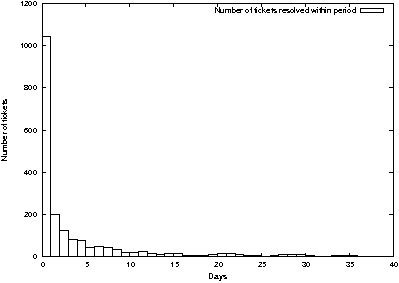
Figure 7: A histogram of the frequency of tickets
resolved in each number of days has a near-exponential
shape.
From the data, we see that requests are multiclass with at least
two distinct classes of requests:
-
A vast majority of requests are resolved quickly (in less than one
month, with a mean time in system of about 3.6 days). Arrival times
for these requests seem to be governed by a sinusoidal non-stationary Poisson process, i.e., arrival rates seem to vary
between a daily high and low on a sine-wave pattern.
-
A small number of requests have an indeterminate and long time in
system. Arrival times for these requests show no discernible structure
(perhaps due to lack of enough examples).
-
The average rate of ticket arrival is gradually increasing over time.
In our case, this seems to be partly due to new faculty hires.
This data also exhibits, however, the main difficulties of
extracting performance statistics from ticket queues:
-
Service times are recorded inaccurately because there is no particular
advantage to recording them accurately. Most tickets are closed late,
because it is not the job of the administrator answering the ticket to
close it, but just to solve the problem. In our case, many tickets are
closed by student staff some time after the problem has been solved.
-
The class of a particular request is not always easily discernible. It
is easier to group requests by time of service rather than class of
problem. In our case, there is a clear distinction between requests
for which an appropriate response is documented, and those for which
an appropriate response is unknown. The former take on average the
same time to resolve, while the latter vary widely.
-
Emergent patterns in the data are only obvious if one is very careful
about correcting for environmental issues. For example, data did not
exhibit a sinusoidal arrival rate until it was corrected for daylight
savings time (DST)!
-
Ticket data does not indicate the severity of a problem. There are no
discernible "flurries" or "bursts" of data for severe problems;
often only one or two people bother to report a major outage.
Other practitioners have mentioned that there are several ways
that request queue data can be biased by operating policy.
-
If people are rewarded for closing tickets quickly, they tend to close
them early, before an actual resolution.
-
If people are rewarded for only the tickets they choose to resolve,
obviously difficult tickets will be avoided.
The final issue plaguing the use of real request queue data is
privacy. Real request data contains flaws in practice. For example,
some requests for which there should be documented scripts remain
undocumented, some requests are forgotten, and some requests can take
an embarrassing amount of time to resolve. For this reason, it is
difficult for researchers to get real data on the nature of requests
and their service times, for sites other than their own.
One lesson learned from our data is the power of good
documentation. If an appropriate response to a problem is documented
or otherwise well known, there seems to be no significant difference
in response time invariant of the nature of the problem. It is
surprising that to a first approximation, differences in service times
for subclasses of requests do not emerge from the data. One
possible reason for this effect is that in these cases, communication
time with clients may dominate the time needed to solve the problem
once it is clearly defined.
Conversely, problems with no documented response wait longer and
may never be solved. At our helpdesk, student staff solve routine
problems and defer only problems with no documented solution to
second-level triage staff. Since the second-level staff are often
planning or deploying new architectures, requests without documented
solutions await their attention and compete with deployment tasks. Of
course, once solved and documented, such a request becomes quickly
solvable.
In our data, a simple pattern emerges. System administration is
composed of a combination of routine tasks and complex troubleshooting
and discovery that borders upon science. Our site's practice is
perhaps best described as a two-class queueing system, with a large
number of routine requests with documented and/or known solutions, and
a smaller number of requests requiring real research and perhaps
development. For the most part, the routine requests are accomplished
by system administrators acting independently, while more complex
requests may require collaboration between system administrators and
take a longer, relatively unpredictable time to complete.
A Simple Model Of Cost
Given the above model of system administration as a queueing
system, we construct a coarse overall model of cost, based upon the
work of Patterson [18] with some clarifications.
First, cost can be expressed as a sum of two components: the
"cost of operations" and the "cost of waiting for changes." The
"cost of operations" contains all of the typical components of what
we normally consider to be cost: salaries, benefits, contracts, and
capital expenditures such as equipment acquisition. For most sites,
this is a relatively predictable cost that remains constant over
relatively long time periods, e.g., a quarter or a year. The "cost of
waiting" is a generalization of Patterson's "cost of downtime",
that includes the cost of waiting for changes as well as the cost of
waiting for outages to be corrected.
While the cost of downtime can be directly calculated in terms of
work lost and revenue lost, the cost of waiting for a change cannot be
quantified so easily. First we assume that R represents the set of
requests to be satisfied. Each request r E R has a cost Cr
and the total cost of waiting is
 We assume that for a request r (corresponding to either an
outage or a desired change in operations), there is a cost function
c r(t) that determines the instantaneous cost of
not accomplishing the change, and times tr1 and
tr2 at which the change was requested and
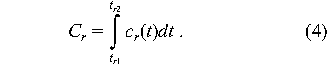
accomplished. Then the tangible cost of waiting is the integral
(running sum) of cr(t) over the waiting period:
We assume that for a request r (corresponding to either an
outage or a desired change in operations), there is a cost function
c r(t) that determines the instantaneous cost of
not accomplishing the change, and times tr1 and
tr2 at which the change was requested and
accomplished. Then the tangible cost of waiting is the integral
(running sum) of cr(t) over the waiting period:
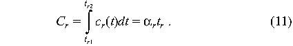
 If as well cr(t) is a constant as
 in Patterson's paper. In general, this may not be true, e.g., if
the change reflects a competitive advantage and the effects of
competition become more severe over time. For example, in the case
of security vulnerabilities, vulnerability is known to increase
over time as hackers gain access to exploits.
in Patterson's paper. In general, this may not be true, e.g., if
the change reflects a competitive advantage and the effects of
competition become more severe over time. For example, in the case
of security vulnerabilities, vulnerability is known to increase
over time as hackers gain access to exploits.
System administrators control very little of the process that
leads to lifecycle cost, but the part they control - how they work
and accomplish tasks - can partly determine the cost of waiting.
In this paper, we consider the effects of practice upon the cost
of waiting in a situation in which the budget of operations is held
constant over some period, e.g., a quarter or a year. Situations
in which cost of operations can vary (e.g., by hiring, layoffs, or
outsourcing) are left for later work.
The cost function cr(t) must model both
tangible (work lost) and intangible (contingency) factors. For
requests concerning downtime, the cost of waiting may be directly
proportional to work and revenue lost, while for requests involving
enhancements rather than downtime, work lost and revenue lost can
be more difficult to quantify. Also, the costs of waiting for
enhancements vary greatly from site to site. For business sites,
delays often incur real revenue loss, while for academic sites, the
effects of delays are more intangible, resulting in missed grant
deadlines, student attrition, and other "opportunities lost". In
the latter case, it is better to model cost as risk of potential
loss rather than as tangible loss.
We can best cope with uncertainty and risk by computing the
expected value of each potential risk. Contingencies are like
requests; they arrive during a period of vulnerability with a
specific rate depending upon the severity of the vulnerability;
these arrivals are often Poisson. The total expected value of an
outage or wait is the sum of expected incident costs, taken over
the various kinds of incidents. If incidents arrive with a constant
Poisson rate , the expected incident
cost is the number of expected incidents times the cost of an
incident. This is in turn a product of the rate of arrival for the
incident, the elapsed time, and the average cost per incident. Note
that the word "incident" applies not only to security problems,
but also to lost opportunities such as students dropping out of
school, employees quitting, etc.
Thus we can think of the cost function cr(t)
for a particular request r as
 where crm(t) represents tangible losses and
cri(t) represents intangible losses. While
crm(t) represents work and revenue losses and is
proportional to the scale of the outage, cri
represents possible losses due to random events. If contingencies
are elements d of a set Dr of all possible
contingencies that can occur during request r, and contingencies
in Dr are statistically independent, then the
cost cri for all of them is the sum of their
individual costs
where crm(t) represents tangible losses and
cri(t) represents intangible losses. While
crm(t) represents work and revenue losses and is
proportional to the scale of the outage, cri
represents possible losses due to random events. If contingencies
are elements d of a set Dr of all possible
contingencies that can occur during request r, and contingencies
in Dr are statistically independent, then the
cost cri for all of them is the sum of their
individual costs
 where crid is the contingency cost for d E
Dr while waiting for r. If contingencies d
E Dr have Poisson inter-arrival times d, then
where crid is the contingency cost for d E
Dr while waiting for r. If contingencies d
E Dr have Poisson inter-arrival times d, then
 where Cd is the average cost per incident for
d. Thus
where Cd is the average cost per incident for
d. Thus
 If crm, d, and Cd
are constants, then
If crm, d, and Cd
are constants, then
 is also a constant, and
Note that there are a lot of if's in the above justification
and the reader should be warned that assumptions abound here. The
formula for cost of waiting simplifies easily only if particular
assumptions hold. As we make these assumptions, our model loses
accuracy and expressiveness. With all assumptions in place, we have
Patterson's model; as he states, it is an oversimplification.
If requests can be divided into classes k E K, each with
a different proportionality constant  ,
then the total cost of processing a set of requests is the total
time spent waiting for each class, times the proportionality constant
for that class. Thus, in the simplest case, the total cost of
waiting is ,
then the total cost of processing a set of requests is the total
time spent waiting for each class, times the proportionality constant
for that class. Thus, in the simplest case, the total cost of
waiting is
 or
or
 Thus the contribution of each class k is proportional to the total time
spent waiting for events of that class.
Thus the contribution of each class k is proportional to the total time
spent waiting for events of that class.
In this approximation we make many simplifying assumptions:
-
Contingencies arrive with Poisson rates.
-
Contingencies are statistically independent of one another.
-
The effect of a contingency does not change over time.
These are limits on how we formulate a problem; we must not
allow dependencies to creep into our classifications. Part of this
formulation is to think of bursts of events as single events with
longer service times. For example, it is incorrect to characterize
"bursty" contingencies such as virus attacks as host events; these
events are not independent of one another. However, the event in which
the virus entered the system is not bursty, independent of all other
like events, and thus can be treated as one contingency.
Likewise, spam from a particular site is not an independent event for
each recipient, though spam from a particular source is often
independent of spam from other sources.
The main conclusion that we make from these observations is that
The intangible cost of waiting for a request is, to a first
approximation, proportional to time spent waiting (though the
proportionality constant may vary by request or request class). While
some constants remain unknown, the values for some proportionality
constants are relatively obvious. If n users are affected by an
outage, then the tangible cost of downtime is usually approximately
proportional to n. Likewise the rate of incidents that involve one
member of the population (such as attrition) is usually approximately
proportional to the number of people involved (due to independence of
people as free agents).
Estimating Service Rates
In the above sections, we show a linear relationship between the
cost of waiting and amount of time spent waiting, and show that the
amount of time spent waiting depends upon arrival rate and service
rate for tasks. In our observation of real systems, arrival rate was
relatively easy to determine. To determine the cost, however, we must
also know the service rate with which requests are completed. We
cannot measure this parameter directly; we can only measure the
waiting time that results from it. How do we estimate the service rate
itself? To answer this question, we borrow from a broad body of work
on complexity estimation in software engineering [19].
Cost modeling in software engineering concerns the cost of
maintaining a large piece of software (such as a program or
configuration script). The basic strategy is to measure the complexity
of the final product in some way, and then predict from that
complexity how much it will cost to craft and maintain the program.
Complexity metrics that can aid in determining cost of a software
engineering project include both "white-box" and "black-box"
methods. A "black-box" method looks at the complexity of
requirements, while a "white-box" method looks at the complexity of
a potential finished product. The goal of either kind of analysis is
to produce a service rate that can be utilized for later analysis. To
map this to system administration, a "white box" method would base
cost estimates on the structure of practice, while a "black box"
approach would base cost estimates upon the structure of the problem.
White-box Methods
In software engineering, white-box software metrics include:
-
Lines of code (LOC): the complexity of a software product is
proportional to its length in lines of code.
-
cyclomatic complexity [16]: the complexity of a piece of software is
proportional to the number of "if" statements in the code.
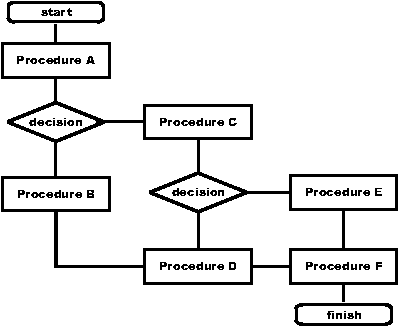
Figure 8: An example troubleshooting
flowchart.
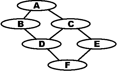
Figure 9: The flow graph corresponding to Figure
8.
It is generally agreed that cyclomatic complexity is a much better
measure of complexity than LOC, for a variety of reasons, including
variations in the expressiveness of programming languages; long
programs in one language can be short in another. The key is to find
something about the program that is more closely related to its cost
than its length. For programs, the number of branches contributes to
the difficulty of debugging or maintaining the program. The key to
white-box analysis of system administration is to find an analogue to
the branches for programs.
Whitebox analysis of programs inspires a similar form of analysis
for system administration procedures. While white-box analysis of
programs starts with pseudo-code, white-box analysis of practice
starts with a recipe or instructions to service a particular kind of
request. If we treat each recipe as a "program", with "branches"
at particular steps, then we can compute the average time taken for
the recipe by keeping statistics on the number of times that
individual steps are utilized in practice. This provides a way to come
up with estimated rates for a procedure, given estimates for subparts
of the procedure.
Note that white-box analysis of a recipe for system administration
is quite different than white-box analysis of a program. In the case
of the program, the white-box measurement of complexity does not
depend upon the input to the program. In system administration, the
performance of a procedure depends upon the nature of the environment.
A white-box estimate of the time needed to service a request is a
measure of both the complexity of the procedure and the complexity of
the environment.
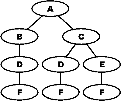
Figure 10: The flow tree corresponding to Figure
9.
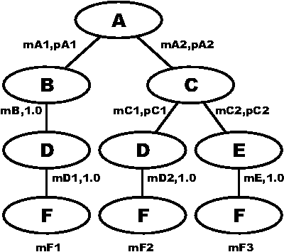
Figure 11: An annotated flow tree tracks statistics
that can be used to compute average completion rate.
One way of performing white-box analysis starts with an (acyclic)
troubleshooting chart for a procedure. We start with a a
troubleshooting chart (Figure 8) that describes procedures to perform
and branches to take after each procedure. We convert this to a flow
graph (Figure 9) by representing only decision nodes. Since a typical
troubleshooting chart has no loops, we convert this graph into a flow
tree by duplicating nodes with two or more incoming edges (Figure 10).
We then annotate branches in that tree with statistics to be collected
or estimated about the branch (Figure 11). These statistics allow us
to compute the mean service rate for the whole tree.
The key to the computation is that given that we know a service
rate for the subtrees of a node in the tree, we can compute the
service rate for the node itself. The nature of the computation is
illustrated in Figure 12. Suppose we know the service rate mB for
subtree B and mC for subtree C. Suppose that we want to compute the
service rate mA for A, and know for each branch out of A, the service
rate for A given that it takes the branch (mA1,mA2) and the probability
with which that branch is taken (pA1,pA2). If we take the branch
from A to B, and A has service rate mA1, then the average service
time for the branch is 1/mA1 + 1/mB.
If we take the branch from A to C, the average service time for the
branch is 1/mA2 + 1/mC.
If we take the branch to B with
probability pA1, and the branch to C with probability pA2, then the
 Thus the average rate is the reciprocal of this.
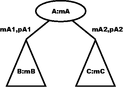
Figure 12: Computing average completion rate for a flow
tree.
To enable this computation, each edge in the program graph is
labeled with two quantities: the mean service rate for the predecessor
of the edge, given that this branch is chosen, as well as the
probability that this branch is chosen. We can either measure these
directly or estimate them by some method. One obvious way to measure
both rates and probabilities is to perform the procedure many times
and record the number of times each node is visited, the average
service time before taking each branch, and the number of times each
branch is taken. Then the ratio of the times the branch is taken,
divided by the times its parent is visited, is the sample probability
that the branch will be taken.
In this abstraction there hides an astonishing fact: the order in
which decisions are made strongly affects the time-in-system for such
a graph. While the rates are properties of the administrative
process, the probabilities of branching are properties of the
environment. Further, these probabilities are not conditional
in the Bayesian sense; they are temporo-conditional in that
they depend upon the previous occurrence of a specific procedure. In
Figure 11, the probability of going to B from A is not the conditional
probability P(B|A), but the probability of B after A: the
probability that we choose B given that A has already been completed.
Bayesian identities do not hold; any change in a procedure affects the
sample probabilities of all branches after it in the script.
One way to estimate branch probabilities in this model is that
certain subtasks depend upon heterogeneity that is routinely tracked.
For example, one step might be to determine whether the affected host
runs Solaris or Linux. In this case, the sample probabilities for the
branches are both known in advance from inventory data. In the same
way, one can estimate some branch probabilities from overall
statistics on the sources of trouble within the network.
Black-box Methods
White-box methods depend upon the fact that the nature of practice
is already known, i.e., we know the steps that people will take to
accomplish tasks. In system administration, as in software, we are
often asked to estimate the cost of a process without knowing the
steps in advance. To do this, we must use a method that estimates cost
based upon the complexity of the outcome rather than the complexity of
the process.
Black-box methods for measuring software complexity include COCOMO
[2, 3, 4]: the complexity of software depends upon an overall
characterization of the software's character and mission. COCOMO
depends upon use of one of two estimations of code complexity:
-
"object points" [3, 4]: the complexity of a piece of software is
proportional to the complexity of the objects it must manipulate.
-
"function points": the complexity of a piece of software is
proportional to the number of functions that it must perform.
The key idea in COCOMO is that there is a relationship between the
cost of maintaining a program and the complexity of its interactions
with the outside world, though we may not know the exact nature of
that relationship in advance. COCOMO is "tuned" for a specific
site by correlating object or function points with actual costs of
prior projects. COCOMO is site-specific; the relationship between
complexity and cost varies from site to site. By computing a ratio
estimating the relationship between requirements and capabilities, one
estimates the time that will be taken to complete requirements.
We can apply the idea of COCOMO to system administration in a very
direct way. While the software model for function points considers
open files, the analogous concept of function points for a network
service would describe that service's dependencies and
interrelationships with others. We know that the number of
dependencies within a service influences the cost of maintaining it;
we do not know the exact relationship.
For example, we might compute the function points for an apache
web server by assigning a number of points to its relationship with
each of the following subsystems: the network (DHCP, DNS, Routing),
the filesystem (protections, mounts), and the operating system (users
and groups). In a function point model, each of these attributes is
assigned a "weight" estimating how difficult it is for a system
administrator to deal with that aspect of configuration and
management. The sum of the weights is then an estimator of "how
complex" the service will be to manage.
The main difficulty with this approach is the number of potential
weights one must estimate; virtually every subsystem mentioned in the
system administrator's book of knowledge [11, 13] has to be assigned a
weight. Further, these weights are not universal; they vary from site
to site, though it is possible that similar sites can use similar
weights. For example, weights assigned to subsystems vary greatly with
the level of automation with which the subsystem is managed.
The cost of providing any service depends not only upon the
complexity of the service, but also upon the capabilities of the
staff. Our next step in defining a function point estimate of the
complexity of system administration is to derive a capability summary
of the administrative staff and site in terms of service rate.
Obviously, a more experienced staff deals with tasks more effectively
than a less experienced one. Capabilities in the model might include
end-user support, service support, architecture, etc. If each staff
member is assessed and the appropriate attributes checked, and a sum
is made of the results, one has a (rough) estimate of capabilities of
one's staff. This has similarities to the SAGE levels of system
administrator expertise defined in the SAGE booklet on job
descriptions [9].
The last step in defining a function point estimate of the
complexity of system administration is to assess the capabilities
maturity of the site itself. One might categorize the site into one of
the following maturity categories [14]:
-
ad-hoc: everything is done by hand.
-
documented: everything is documented, no automation.
-
automated: one can rebuild clients instantly.
-
federated: optimal use is made of network services.
Again, each one of these has a weight in determining the overall
capabilities. The sum of administrator capabilities and site
capabilities is an estimate of overall "capability points" for the
site.
It can then be argued that the complexity of administering a
specific subsystem can be estimated by a fraction
 where
service points and capability points
are sums of weighted data as described above. If the weights for
capability points are rates in terms of (e.g.) service-points per
hour, then the complexity is the average response time in hours to a
request.
where
service points and capability points
are sums of weighted data as described above. If the weights for
capability points are rates in terms of (e.g.) service-points per
hour, then the complexity is the average response time in hours to a
request.
The overwhelming problem in tuning COCOMO for system
administration is that tuning the model requires detailed data on
actual measured rates. The tuning process requires regression to
determine weights for each of the complexity and quality factors. This
is accomplished by studying a training set of projects with known
outcomes and properties. To use COCOMO-like systems, we must be able
to gather more accurate data on the relative weights of subsystems
than is available at present.
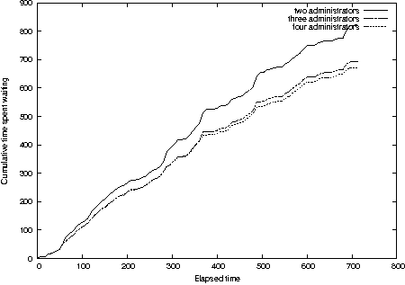
Figure 13: Diminishing returns when adding
administrators to a queue.
Some Experiments
So far, we have seen that we can estimate the cost of system
administration via one of two models. "Black box" methods require
that we assess the time impact of the complexities of the problem
being solved, while "white box" methods require that we estimate the
time taken for a detailed set of tasks. Of these methods, "black
box" methods give us information more quickly, but these methods
require that we "score" facets of the problem being solved as harder
or easier than others. These scores must be developed via practice,
but we can learn something about the relative complexity of black-box
attributes via simulation. By simulating practice, we can account for
realistic human behaviors that cannot be analyzed via known queueing
theory. We can also observe how real systems can potentially react to
changes in a less ideal way than ideal queueing models suggest.
Particularly, we can study behavior of queueing systems "on the
edge"; almost out of control but still achieving a steady state. In
our view, this situation describes more IT organizations than it
should.
The Simulator
The simulator, written in C++, is basically an M/M/c queue
simulator with the ability to simulate non-ideal ("non-product")
behaviors. It assumes that we have c identical system administrators
working 24x7 and generates a variety of requests to which these ideal
administrators must respond. One can vary the behavior of the system
administrator and the request queue and measure the results. The input
to the simulator is a set of classes of tasks, along with arrival and
service rates for each task. The output is the time spent waiting for
requests (by all users), both per time-unit of the simulation and
overall. We assume for this simulator that the cost of waiting is a
constant; a unit wait by a single individual results in some constant
intangible cost. These simulator assumptions are very much less
complex than real practice, but one can make some interesting
conclusions from even so simple a model.
Diminishing Returns
Our first simulation exercise is to study the effects of adding
system administrators to a group servicing simple requests. We set up
a simple multi-class system with a varying number of system
administrators all of whom have identical average response rates.
There are four request classes, corresponding to requests whose
service time is an average of 1, 3, 8, and 24 hours, respectively. The
service rate of each request class is twice its arrival rate, creating
a balance between arrivals and service. We ran the exact same
simulation for two, three, and four system administrators. The
cumulative time spent waiting for service is shown in Figure 13. There
is clearly a law of diminishing returns; the change in wait time from
three to four system administrators does not significantly change the
time spent waiting for service.
Saturation
Realistic system administration organizations can be faced with
request volume that is impossible to resolve in the time available.
We know from classical queueing theory that an M/M/c queuing
system exhibits predictable response time only if /c
< 1, where is the arrival
rate, c is the number of administrators, and is the service rate per administrator. In
other words, there has to be enough labor to go around; otherwise
tickets come in faster than they can be resolved, the queue grows,
and delays become longer and longer as time passes.
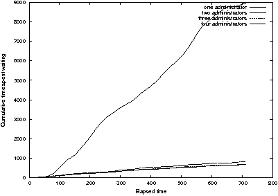
Figure 14:
One administrator performs very poorly compared to two, three, and
four.
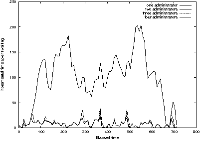
Figure 15: Incremental data for Figure 14 shows
that utilizing one administrator leads to chaotic wait times.
Figure 14 shows the same simulation as before, but adds the case
of one administrator. This seems like an unbalanced situation in which
request rate is greater than service rate, but looking at waiting time
per unit time (Figure 15) we see that waiting time is not always
increasing with time. So although one administrator is very much
slower than two or three, the situation is not completely out of
control. Note, however, that the situation of the single administrator
is very sensitive to load; he is "on the brink of destruction."
Small changes in load can cause large variations in response time, and
the cost of administration due to waiting is "chaotic", especially
when a request when a long service time enters the queue.
Nevertheless, on average, the time spent waiting varies directly with
elapsed time of the simulation.
Figure 16 shows incremental waiting time for a truly "saturated"
system in which there is no way for administrators to ever catch up.
We saturate the queue in the previous example by multiplying the
arrival rates for all requests by four. In this case, one and two
administrators are in trouble; queue length is growing linearly with
time along with wait time. Figure 17 shows the cumulative time for
this example. In a saturated queueing system, since time spent waiting
increases linearly with elapsed time, the cumulative time spent
waiting varies as the square of elapsed time.
Brinksmanship
We consider it a fair statement that many IT organizations run
with /c
quite close to 1. It is thus no surprise that it is very difficult
for these organizations to cope with changes that might increase
load upon system administrators, even for a short time.
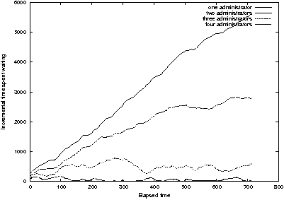
Figure 16: Multiplying the arrival rate by four
overloads one or two system administrators.
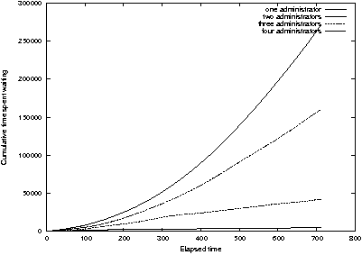
Figure 17: Cumulative wait time for overloaded system
administrators varies as the square of elapsed time.
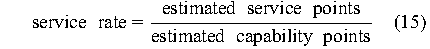
There is a solution, but it is counter-intuitive. Figure 18 shows the
effect of a "catastrophic" flurry of requests arriving in a near-saturated system. For a short while, wait times go way up, because the
system is already almost saturated and the new requests push it over
the limit. The key is to distribute the same requests over a long time
period (Figure 19), to avoid pushing the system over the limit and
save waiting time. Note that in both figures, one administrator alone
simply cannot handle the load and chaotic waits occur in both cases.
Lessons Learned
Human systems self-organize around maximum efficiency for the task
at hand, but not necessarily for future tasks. As such, we as system
administrators are often near the "saturation point" in our
practice. As in Figure 18, small increases in load can lead to
catastrophic delays. But the strategies in Figure 19 can help.
One part of coping with being understaffed is to utilize
automation to lessen workload, but that can lead to queue saturation
in an unexpected way. The quandary of automation is that when
something goes wrong, it is not one host that is affected, but
potentially hundreds. If an automation mistake affects hundreds of
nodes, we often have the situation in Figure 18; there are hundreds of
questions to answer and the queue is already saturated. These
questions can be as simple as educating users about a different
command for invoking software; it takes little perturbation to
saturate a queue that is already nearly saturated. The worst possible
case is that automation uncovers latent pre-existing conditions that
cause failures. In this case, troubleshooting may take a large amount
of time while the queue fills.
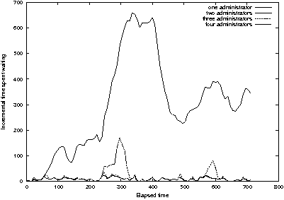
Figure 18: A flurry of 100 requests causes a
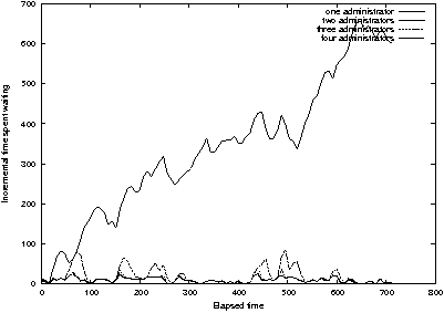
Figure 19: Distributing the 100 requests in Figure 18
over a longer time interval improves wait times except for an
administrator working alone.
The main lesson of this paper is that staged deployment is often
better than large-scale automated deployment, when system
administrators are near saturation. It is often far better to control
the request queue by upgrading a small number of users at a time,
rather than risk a flood of potentially unmanageable requests due to a
massive upgrade. If a massive upgrade is required, extra staff are
needed to handle the load through the upgrade period. It is no shame
to ask for help when the alternative is that your organization loses
much more money than it would spend as a result of hiring help.
Open Questions
Obviously, this paper is a very small step toward understanding
the effects of practice upon cost. Simulations are no replacement for
real measurements, and real measurements remain impractical. We end
this study with more questions than when we started.
First, there are at least a hundred factors affecting the practice
that we are not simulating. Some have peripheral effects, such
as human learning; we were surprised at how little an effect it has
when running simple simulations. Others have major effects, such as
peer mentoring, user conditioning, and error propagation. Models of
user behavior (such as those described in [12]) have not been
incorporated here, nor have we incorporated behavioral aspects such as
conditioning to pre-existing circumstances. For example, it is common,
in the presence of poor response time, for users to stop making
requests and go elsewhere for help. Likewise, events and incidents are
often not independent of one another; requests can be bursty or
sparse. Like Patterson's paper, this one also oversimplifies a complex
problem, giving slightly more sophisticated methods than the "back of
an envelope" to estimate the results of very complex processes.
Second, we should not forget the wealth of work on queueing
systems upon which we can draw. Reference [10] analyzes the properties
of sinusoidal arrivals - like the ones we observed - and gives a
method for computing the number of servers that are needed to achieve
best-case performance. Can these methods be used to analyze system
administration? The burning question is what can we afford to idealize
and for what must we account by simulating realistic practice.
Simulations are particularly difficult to use for asking "what-if"
questions because realistic answers require the results of thousands
of runs to be averaged.
Integrating Measurement with Practice
One of the largest blockades against understanding the cost of
practice is that the activity of cost measurement is separate from
that of practice. Can we integrate this with practice? Could we
develop tools that - by their use - provided input data to a cost
model? This approach seems to have some promise.
Imagine a tool that - when you utilize it - keeps records on how
long the task takes. Imagine this database being used to populate a
function point model, so that the complexity of specific tasks can be
accurately predicted. If done correctly, this would make the cost
analysis intrinsic, transparent, and completely invisible to the
practitioner. It should neither limit nor delay the practitioner, but
should keep track of realistic time estimates for specific tasks.
One idea is that of a "smart troubleshooting guide" that keeps
records on how long was spent on each procedure. While the
administrator was following a procedure, this guide would record time
spent on each page and in each procedure, for the purpose of recording
how long, on average, each procedure takes.
Of course, the large question here is not that of efficiency or
transparency but that of privacy. Any mechanism that measures our
practice also keeps data that we might not want to be stored, such as
individual performance records. As well, the potential exists for this
data to be misused in ways that damage the profession; e.g., punishing
administrators who are "slower" but consistently make fewer errors.
Conclusions
No simulator or model is a perfect substitute for reality. In this
paper, we have studied some of the easiest ways to obtain predictions
about the cost of system administration, when it is considered to be a
sum of infrastructure cost and an indirect cost proportional to time
spent waiting. They are of course not particularly accurate, but are
they accurate enough to use in making intelligent decisions?
One lesson to take from software engineering is that often an
educated guess is better than no information at all. Even if we get
within an order of magnitude of estimating the cost of managing a
particular service, we know more than when we started, and can tune
that figure by observing practice. The first step is to get real data.
And this process cannot wait. At this time, the profession is
"under siege" from those who would eliminate system administration
as a profession. The grand promise of autonomic computing, however, is
not easy to obtain, and the cost justifications of the technology
often do not include an analysis of the cost of troubleshooting when
things go wrong. By understanding the cost of our practice, we can
better respond to arguments claiming superiority of autonomic
computing methods, and be able to realistically compare human-centered
and machine-centered styles of system administration.
This is a very small step in a new direction. If it has sensitized
practitioners to the idea that waiting time matters, it has
accomplished its goal. The best models and measurements for analyzing
indirect costs are yet to be discovered. But if the reader is - like
many of us - near saturation, one can modify one's practice to ease
the pain, not by applying automation blindly, but by strategically
planning changes so that requests do not become overwhelming. This is
the first step toward a practice in which queues never saturate and IT
managers understand the difference between under-utilization and
required capacity in system administration organizations. System
administrators are like insurance; a properly functioning organization
does not have them all busy all of the time, except during contingency
periods.
Acknowledgements
As usual, this work was a product of collaboration among a broader
community of learning than the authors. Paul Anderson, Mark Burgess,
and many others nudged the authors toward developing their model more
carefully. The systems staff at Tufts University ECE/CS graciously
donated their time and ticket queue for study; John Orthoefer was
particularly helpful in helping us obtain data. Marc Chiarini worked
long hours to offload the authors from other tasks during writing and
to proofread the document.
Author Biographies
Alva L. Couch was born in Winston-Salem, North Carolina where he
attended the North Carolina School of the Arts as a high school major
in bassoon and contrabassoon performance. He received an S.B. in
Architecture from M. I. T. in 1978, after which he worked for four
years as a systems analyst and administrator at Harvard Medical
School. Returning to school, he received an M.S. in Mathematics from
Tufts in 1987, and a Ph.D. in Mathematics from Tufts in 1988. He
became a member of the faculty of Tufts Department of Computer Science
in the fall of 1988, and is currently an Associate Professor of
Computer Science at Tufts. Prof. Couch is the author of several
software systems for visualization and system administration,
including Seecube (1987), Seeplex (1990), Slink (1996), Distr (1997),
and Babble (2000). He can be reached by surface mail at the Department
of Computer Science, 161 College Avenue, Tufts University, Medford, MA
02155. He can be reached via electronic mail as couch@cs.tufts.edu.
Ning Wu is pursuing his Ph.D. at Tufts University. His research
interests are in system management, wireless ad-hoc networking,
security, and P2P systems. Before studying at Tufts, he had worked as
an engineer for Genuity and Level 3 Communications Inc. He received an
M.S. from State University of New York at Albany, an M.E. from East
China Institute of Computer Technology, and a B.S. from Southeast
University in China. Ning can be reached via email at
ningwu@cs.tufts.edu.
Hengky Susanto is a computer science Ph.D. student at Tufts
University. His research interests are in Autonomic computing, System
Management, and Networking Area. He also worked as a software engineer
at EMC and StorageNetworks Inc prior to returning to school. He
received a B.S from University of Massachusetts at Amherst and a M.S
from University of Massachusetts at Lowell, both in computer science.
Hengky can be reached at hsusan0a@cs.tufts.edu.
References
[1] Apthorpe, R., "A Probabilistic Approach to Estimating Computer
System Reliability," Proc. LISA 2001, USENIX Assoc., 2001.
[2] Boehm, Barry, "Anchoring the Software Process," Barry
Boehm, IEEE Software, July, 1996.
[3] Boehm, Barry, Bradford Clark, Ellis Horowitz, Ray Madachy,
Richard Shelby, and Chris Westland, "Cost Models for Future Software
Life Cycle Processes: COCOMO 2.0," Annals of Software
Engineering, 1995.
[4] Boehm, Barry, Bradford Clark, Ellis Horowitz, Ray Madachy,
Richard Shelby, and Chris Westland, "COCOMO 2.0 Software Cost
Estimation Model," International Society of Parametric
Analysts, May, 1995.
[5] Burgess, Mark, "Theoretical System Administration,"
Proc. LISA 2000, USENIX Assoc., 2000.
[6] Burgess, Mark, Analytical Network and System
Administration: Managing Human-Computer Systems, Wiley and Sons,
2004.
[7] Couch, Alva and Paul Anderson, "What is this thing called
system configuration," an invited talk to LISA-2004, USENIX Assoc.,
2004.
[8] Cowan, et al., "Timing the application of security patches
for optimal uptime," Proc. LISA 2002, USENIX Assoc., 2002.
[9] Darmohray, T., Ed, Job Descriptions for System
Administrators, Revised Edition, SAGE Short Topics in System
Administration, USENIX Assoc.
[10] Eick, S. G., W. Massey, and W. Whitt, "Mt/G/ queues with sinusoidal arrival rate," Management Science 39,
Num. 2, 1993.
queues with sinusoidal arrival rate," Management Science 39,
Num. 2, 1993.
[11] Halprin, G., et al., "SA-BOK (The Systems Administration
Body of Knowledge)," https://www.sysadmin.com.au/sa-bok.html.
[12] Haugerud, Harek and Sigmund Straumsnes, "Simulation of
User-Driven Computer Behaviour," Proc. LISA 2001, USENIX
Assoc., 2001.
[13] Kolstad, R. et al., "The Sysadmin Book of Knowledge
Gateway," https://ace.delos.com/taxongate.
[14] Kubicki, C., "The System Administration Maturity Model -
SAMM," Proc. LISA 1993, Usenix Assoc., 1993.
[15] Maekawa, M., A. Oldehoeft, and R. Oldehoeft, Operating
Systems: Advanced Concepts, Benjamin/Cummings, 1987.
[16] McCabe, T. J., and C. W. Butler, "Design Complexity
Measurement and Testing." Communications of the ACM, Vol. 32,
Num. 12, pp. 1415-1425, December, 1989.
[17] Menasce, David, Performance by Design: Computer Capacity
Planning by Example, Prentice-Hall, 2004.
[18] Patterson, David, "A simple model of the cost of
downtime," Proc. LISA 2002, USENIX Assoc., 2002.
[19] Pressman, Roger S., Software Engineering: A
Practitioners' Approach, Fifth Edition, McGraw-Hill, 2001.
|