4th USENIX Symposium on Networked Systems Design & Implementation
Pp. 115–130 of the Proceedings
A Location-Based Management System for Enterprise Wireless LANs
Ranveer Chandra, Jitendra Padhye, Alec Wolman, Brian Zill
Microsoft Research
Abstract: The physical locations of clients and access points in a wireless LAN may have a large impact on network performance. However, today’s WLAN management tools do not provide information about the location of clients apart from which access point they associate with. In this paper, we describe a scalable and easy-to-deploy WLAN management system that includes a self-configuring location estimation engine. Our system has been in operation on one floor of our building for several months. Using our system to observe WLAN usage in our building, we show that information about client locations is crucial for understanding WLAN performance. Although WLAN location systems are a widely studied topic, the novel aspects of our location system primarily relate to ease of deployment. The main contribution of this paper is to show the utility of office-granularity location in performing wireless management tasks.
1 Introduction
Wireless LANs (WLANs) are an important part of today’s enterprise networks. However, end users typically do not enjoy the same level of service from WLANs that they have come to expect from wired networks. Better tools for managing WLANs are required for improving the reliability and the level of service provided by today’s WLANs.
Wireless networks are fundamentally different from wired networks, in that the behavior of the network is location-dependent. Due to the nature of wireless signal propagation, the physical location of both the transmitter and the receiver may have a large influence on the performance observed by end-users. Specifically, the probability of frame loss, and the data rate selected for frame transmission can be impacted by the locations of the transmitter and the receiver.
The need for incorporating location information in WLAN management tools is also reflected in the common questions asked by administrators of WLANs: Is the access point (AP) placement adequate for serving the locations from where my network is most actively used? Are there areas in my network where clients consistently experience poor performance? How does the distance between an AP and a client affect client’s performance? Are there areas that have no coverage at all? With answers to these questions, network administrators can take concrete steps to improve the reliability and performance of their networks.
The WLAN management and monitoring systems available today can not satisfactorily answer these questions. The reason is that many of them provide no information about client’s location at all [26, 12]. Others [8, 21, 18] simply approximate the location of the client with the location of the AP that the client is associated with. Our data shows that in our network, 25% of active clients do not associate with the nearest AP. Consequently, these systems can not accurately characterize the influence of location on client performance.
We note that there has been a lot of research on accurate location estimation using WLAN technologies [7, 23, 22, 30, 17]. We believe that the primary reason that these technologies are not integrated with today’s WLAN monitoring systems is that the location estimation techniques are generally not easy to deploy. Many location systems require a mapping step whereby an administrator walks throughout the area being covered by the location system to create a “profile” of the environment. Moreover, this profile needs to be updated at regular intervals to ensure that it reflects the current environment.
We have designed and implemented a WLAN management system with an integrated, self-configuring indoor location system. Our location system is accurate to the granularity of individual offices and requires minimal manual intervention to setup and operate.
Our system is built upon the DAIR platform described in [6, 5]. The DAIR platform turns ordinary user desktops into wireless monitors (AirMonitors) by attaching a wireless USB dongle to each of them. The DAIR architecture allows us to create a dense deployment of WLAN monitors in a scalable and cost-effective manner.
The dense deployment of AirMonitors has several advantages. In most cases, there is at least a single AirMonitor that can hear a majority of the packets flowing between a given client and its AP in a single direction (another Air-Monitor may hear most of the packets flowing between the client and the AP in the other direction). This allows us to sidestep the complex tasks of trace merging and fine-grained time synchronization faced by other WLAN monitoring systems [26, 12]. The dense deployment also allows us to use very simple location estimation algorithms, yet achieve office-level accuracy.
We have deployed this system in our building over the last six months. Our current deployment consists of 59 AirMonitors, and covers an entire floor. We have been using it to monitor the WLAN in our building. During this time, our system was able to answer many of the questions we posed earlier. For example, we detected that clients in one corner of our building received consistently poor performance. We were able to provide a fine-grained characterization of the workload on our network: we noticed that clients located in people’s offices tend to download more data than clients located in various conference
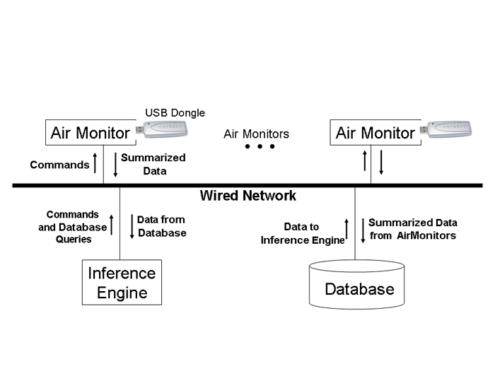
Figure 1: The DAIR Architecture.
rooms. We characterized the impact of distance on uplink and downlink transmission rates as well as loss rates in our environment. Much to the delight of system administrators, we also located transmitters that were sending malformed 802.11 packets. We discovered and reported a serious misconfiguration shortly after new APs were deployed on our floor. These APs sent downlink traffic at 5.5Mbps, regardless of the location of the client. This problem has since been fixed.
In summary, the key contributions of our paper are:
-
To the best of our knowledge, we are the first to integrate office-level location accuracy into a WLAN management system.
-
We show that correlating client locations with a variety of performance metrics yields new insights into WLAN behavior.
-
We demonstrate the usefulness of our system by using it to monitor an operational WLAN.
-
We show that by using a dense deployment of wireless sensors, one can significantly simplify the tasks of wireless monitoring and location estimation.
2 The DAIR Platform
The design and the architecture of the DAIR system has been described in detail in [5]. Here, we provide a brief review of the system architecture.
The DAIR system is designed for easy and inexpensive deployment in enterprise environments. Existing desktop machines serve double-duty as WLAN monitors. The IT department can mandate which desktops perform this service, and they can also manage the process of deploying the DAIR software on these systems.
Figure 1 provides a high-level illustration of the three major components of the DAIR system: the AirMonitors; the database server; and the inference engine. We use the term AirMonitor to refer to ordinary desktop computers in the enterprise that are equipped with inexpensive USB 802.11 wireless cards and have two components of the DAIR software installed: (1) the AirMonitor service; and (2) a custom device driver that works with USB wireless cards based on the Atheros chipset. The AirMonitor service is user-level code that runs as a Windows service, the equivalent of a daemon on Unix systems. The device driver customizations allow the wireless card to receive all 802.11 frames, including those destined for other 802.11 stations and those with decoding errors.
The AirMonitor service contains all of the user-level code for monitoring. It enables packet logging at the driver level, at which point all frames are delivered to the service. Within the service, the basic unit of extensibility is a “filter’: each new application built to use the DAIR system installs an application-specific filter that runs inside the AirMonitor service. Each frame from the driver is delivered to all running filters. The filter’s primary task is to analyze the frames, summarize them in an application-specific manner, and then submit those summaries to the database server.
The intent is that filters do whatever summarization is sensible to improve the scalability of the system without imposing an undue CPU burden on the AirMonitors – we don’t want to submit every frame that each AirMonitor overhears to the database, yet we also don’t want the Air-Monitors to do all of the complex data analysis, which is the responsibility of the inference engine. While the precise definition of what constitutes undue burden varies based on circumstances, parameters such as history of CPU and memory usage are taken into consideration [14].
We use Microsoft’s SQL Server 2005 as our database server. We made no custom modifications to the database server. The DAIR system is designed to scale to handle very large enterprises. When the number of AirMonitors in the system exceeds the capacity of a single database server, one can simply deploy another database server. However, AirMonitors should be assigned to servers in a location-aware manner, to limit the number of queries that must be performed across multiple database servers.
The computationally intensive analysis tasks are all performed by the inference engines. Inference engines are stand-alone programs that analyze the data gathered by the AirMonitors. The inference engines learn about new events by issuing periodic queries to the database server.
3 Management System Design
In this section, we describe the new infrastructure components, beyond the original DAIR platform described in our previous work, that are utilized by all of our wireless management applications.
3.1 Location engine
The goal of our location engine is to determine the location of any 802.11-compatible transmitter (which includes WLAN clients such as laptops and hand-held devices) on our office floor, and to communicate that location to the rest of the management system. Our design was guided by the following set of requirements.
First, we require no cooperation from the clients: no special software or hardware is needed, and the clients need not communicate directly with the location system.
Second, the location system should provide “office-level” accuracy: the error should be within 3 meters, approximately the size of a typical office. Although other proposed location systems provide greater accuracy, this level is sufficient for our needs. Third, to ensure easy deployment, the system must be self-configuring – it cannot require manual calibration. Finally, the location system must produce output in a way that is physically meaningful to the network administrators, which precludes having the system construct its own virtual coordinate space as Vivaldi does [13].
The basic idea behind our location system is similar to that of many previous 802.11-based location systems. The AirMonitors record the signal strengths of frames transmitted by a sender. This information is combined with the known AirMonitor locations to estimate the location of the transmitter. The key distinguishing features of our location system are: 1) by deploying AirMonitors with high density, we can avoid the manual profiling step required by previous indoor 802.11 location systems [7, 17]; and 2) we use external sources of information commonly available in enterprises environments to automatically determine the location of most AirMonitors.
In the remainder of this section, we describe the bootstrapping method for automatically determining the Air-Monitor locations, followed by the three simple location estimation algorithms supported by the location engine.
3.1.1 Determining the AirMonitor Locations
To automatically determine the physical location of the AirMonitors, we start by determining the number of the office that each AirMonitor is located in. Because the DAIR system uses end-user desktops for the AirMonitors, we can analyze the login history of these machines to determine who the primary user is. In a typical enterprise, the occupant of an office is generally the primary user for the machines in that office. We examine the system event-log for user login and console unlock events, and extract the user identifier for these events. We ignore remote login events and non-console unlock events. We then determine the primary user by selecting the user with the most login and unlock events in a given time period. With this information, we then consult a database of users and office numbers (our implementation uses the Microsoft Active Directory service [27]) to determine the office number where the machine is likely located.
The final step uses online to-scale building maps, which are available to us in Visio XML format. The map includes labels for the office numbers, which are centered within each office. We parse the XML, determine the graphical coordinates of each label, and convert these to the physical coordinates. This procedure gives us an estimate of the center of each office. By combining this information with the user-to-office mapping, we can automatically determine the location of most of our AirMonitors.
The details of this procedure are clearly specific to our particular environment. Although we believe that many enterprise environments maintain similar types of information, the specific applications and data formats may differ. Also, even in our environment these techniques are not completely general. For example, this procedure tends not to work well for machines located in public spaces, such as conference rooms and lounges, because the login history on these machine does not tell us much. For such machines, we still must manually inform the system of the office number to get the coordinates into our database.
Our assumption that the AirMonitor location is in the center of each office is another source of error. We do not try to pinpoint the location of an AirMonitor within an office because doing so would require significant manual effort. This approximation is appropriate for us because we only require office-level accuracy. We assume that the physical location of AirMonitors does not change often. We determine the location of the AirMonitor when we first deploy it and re-confirm it only infrequently.
3.1.2 Locating a Transmitter: StrongestAM
During the course of their normal operation, various Air-Monitors hear the frames sent by the transmitter, which we identify by the sender MAC address. On a periodic basis, the AirMonitors submit summaries to the database of the signal strength of those frames overheard. These summaries contain start and end timestamps, the AirMonitor identifier, the sender MAC address, the channel on which the frames were heard, the number of frames sent by this transmitter, and the total RSSI of those frames.
When the inference engine wants to locate a client, it provides the start and end time and the sender MAC address to the location engine. The location engine computes the average signal strength seen by each AirMonitor during the specified time period for that transmitter. Then, it chooses the AirMonitor that saw the highest average RSSI (i.e. strongest signal strength) during this period and reports this AirMonitor’s location as the location of the client.
The StrongestAM algorithm is very simple, and is likely to give inaccurate results in many cases. One reason is that even when a client is stationary, the RSSI seen by the AirMonitors can fluctuate significantly. Some of these fluctuations are masked due to averaging over multiple packets. Yet, if two AirMonitors are reporting roughly equal signal strength, the fluctuations may make it impossible to pick the strongest AM without ambiguity.
However, if the AirMonitor density is high enough, this simple algorithm might suffice to provide office-level granularity in most cases. As we will show later, this algorithm works well primarily when the client is located in an office where we do have an AirMonitor.
3.1.3 Locating a Transmitter: Centroid
The next algorithm we implemented, Centroid, is a variant on the StrongestAM: instead of selecting only the strongest AirMonitor, we select all AirMonitors whose average RSSI is within 15% of the average RSSI of the strongest AirMonitor. We then report the client location as the centroid of the set of selected AirMonitors. If there are no AMs within 15% of the strongest AM, the location is just reported to be that of the strongest AM.
This algorithm has several attractive features, especially in our deployment, where we have an AirMonitor in about half of the offices on our floor. When the transmitter is in the same office with an AM, it is generally the case that this AM sees significantly higher RSSI values, compared to all other AMs. As a result, the office is correctly picked as the location of the transmitter, without any adjustment. Also, the accuracy of this algorithm is not affected by the moderate adjustments in transmit power that are seen when clients use transmit power control. If a packet is sent at a lower power level, all the AMs will see a proportional decrease in the observed RSSI.
In addition, the Centroid algorithm is unaffected by small fluctuations in the RSSI that various AirMonitors report. The threshold implies that the set of AMs that we compute the centroid over does not change with small fluctuations in reported signal strength.
The Centroid algorithm does have one drawback. If the set of AirMonitors we compute the centroid over are all on one side of the actual client location, we could see a significant error. As it turns out, this is not a significant problem in our deployment but it certainly could be in other environments. We discuss the issue more in Section 5. To address this problem, we developed a third algorithm which we discuss next.
3.1.4 Locating a Transmitter: Spring-and-ball
The previous two algorithms do not explicitly take into account the radio propagation characteristics of the local environment. Our third algorithm, Spring-and-ball (inspired by Vivaldi [13]), addresses this problem by using “profiles” of the area in which the WLAN is deployed.
A profile is an approximate, compact representation of how the signal strength degrades with distance in the local environment. To generate a profile, each AirMonitor broadcasts special probe packets at regular intervals, that contain the identity of the transmitting AirMonitor. The other AirMonitors record these probe packets and report the average signal strength of packets heard from each AirMonitor to the central database. Using the known distance between two AirMonitors and the observed average RSSI between those AirMonitors, the inference engine fits a set of simple curves to the combined observation data, and picks the best fit as the profile of the environment. The resulting profile is labeled with the channel on which the probe packets were sent and stored in the database.
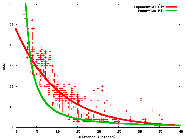
Figure 2: Sample profile data and two fitted curves.
We currently consider linear, exponential, logarithmic, and power law curves. Each of these curves can be fitted using variants of the least-squares fitting method. We do not filter the raw data in any way; all points are considered while determining the fit. The goodness of fit is determined by the R2 (correlation coefficient) value. An example is shown in Figure 2.
When the location engine is asked to locate a client, it computes the average signal strength that each AirMonitor observed. It then calculates the initial estimate of the location using the Centroid algorithm. The estimate is the refined using a Spring-and-ball algorithm as follows.
We select the most recent profile that matches the frequency band
of the channel on which the packets were heard. Using the profile,
we calculate the signal strength that each AirMonitor should have
seen had the transmitter been at the estimated location.
If the calculated signal strength value is less than 0, it is assumed to be 0. Similarly, if the calculated signal strength value exceeds 100, it is assumed to be 100.
We then consider the difference
between the calculated signal strength and the signal strength that the
AirMonitor actually observed.
The absolute value of the difference corresponds to the magnitude of the force on the ”spring” that connects the transmitter to the AirMonitor. The sign of the difference indicates whether the spring is compressed or stretched. The direction of the force is along the line connecting the AirMonitor location to the estimated transmitter location.
We then move the estimated location of the transmitter a short distance in the direction of the cumulative force.
If either the X or the Y co-ordinate of the location falls outside the boundary of the floor, it is adjusted to be within the boundary.
This reduces the magnitude of the error by a small amount. This is the new estimated location of the client. We recalculate the forces at this new location, and repeat the process until one of the following is true: (i) 5000 iterations have elapsed, (ii) the magnitude of the error falls below 0.1, or (iii) the force at the new location exceeds by 10% the minimum force seen so far.
The Spring-and-ball algorithm will converge to a global minimum only when the magnitude of the force is linearly proportional to the distance [13]. This is not true in our setting, since the drop in signal strengths is not linearly proportional to the distance. However, we have found that the algorithm works well in practice.
This algorithm overcomes the key limitation of the Centroid algorithm. If all the AirMonitors that hear a particular client are on one side, the Centroid algorithm would pull the client to be in midst of those AirMonitors. The Spring-and-ball algorithm will realize that the signal strengths reported by the AMs are too low to be coming from the central location, and will push the client to the correct side.
The key challenge in implementing the Spring-and-ball algorithm is the generation of profiles. Questions that arise include: How often should profiles be generated (i.e. do time-of-day effects create significant errors)? What type of curve should we use to fit the data? We have carried out extensive experimental sensitivity analysis of the Spring-and-ball algorithm. We have found that the time of day effects do not significantly impact the accuracy. In fact, we only generate new profiles when we add new Air-Monitors to the system. We have also found that either a log or power curve provides a good fit to the observed data. We do not describe the results of our study further, because we want to focus our results on the use of the location system for management applications.
Some of the previous WLAN location estimation systems proposed in the literature are more accurate than our system. Our goal, however, was to design a location system that provided office-level accuracy, and that met our rather stringent requirements for ease of deployment.
3.2 AP Tracking
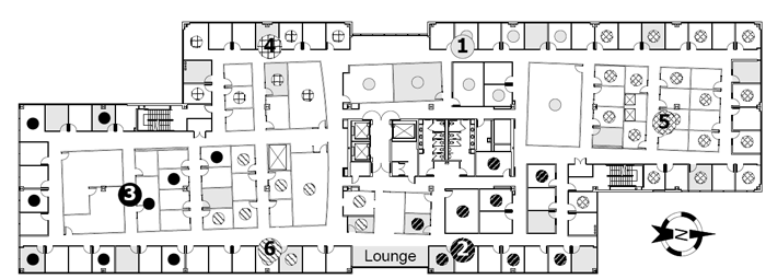
The corporate APs in our building are controlled by a central server [3], which dynamically reconfigures which channels the APs operate on. The frequency of change depends on a variety of factors, including traffic load. We have observed some of our APs changing channels as many as six times in a 12 hour period. As a result of this dynamic channel assignment, we can not assign our AirMonitors to listen to fixed channels. Instead, each Air-Monitor is assigned to track the nearest AP – this configuration is shown in Figure 3.
The AirMonitor implements AP tracking by continuously looking for beacons sent by the assigned AP. If no beacons are observed during a 10-second period, the Air-Monitor goes into scanning mode, where it listens for beacons for 150 ms on each of the 11 channels in the 2.4 GHz band, until the assigned AP is heard from again. If scanning fails to find the assigned AP within two minutes, it goes back to the previous channel where it heard the AP, on the assumption that the AP may have failed. Every 30 minutes, it re-enters scanning mode and looks for the AP on the other channels. While in scanning mode, packet delivery to all the filters is suspended.
3.3 Address Matching
The frame format of the 802.11 standard is not fully self-describing. One example of this is that there are two types of 802.11 frames, namely the CTS (clear-to-send) and ACK (acknowledgment) frames, that do not contain the MAC address of the device that transmits those frames. This means that for devices using promiscuous mode to passively listen to 802.11 conversations, they cannot directly determine who sent those packets. Fortunately, if the passive listener is capable of overhearing both directions of the conversation, then it is possible to infer the address of the transmitter of such frames.
One component of the AirMonitor service is responsible for inferring and then filling in both the transmitter and BSSID fields for both CTS and ACK frames. This information is filled in before the frame is handed off to any other filters that are running on the AirMonitor, and therefore these filters can simply assume that this information is available whenever matching was possible.
The strategies we use to infer the transmitter are different for ACK frames than for CTS frames. To determine the transmitter of an ACK frame, we need to analyze packets that arrive back-to-back. If the first frame type is a Data or Management frame, then we remember the value of the Duration header for that frame. When the next frame arrives, we determine if it is an ACK frame that has arrived within the time period allocated by the previous frame. If so, then we know that the receiver of the first frame must be the transmitter of the ACK frame. Furthermore, we use the ToDS and FromDS bits in the header of the previous frame to determine the correct BSSID to attribute to this ACK frame.
To infer the transmitter for CTS frames, we considered using a similar strategy where the previous frame should be an RTS frame. However, in our network the vast majority (more than 99%) of CTS frames are “CTSto-self” frames that are used for 802.11g-mode protection. In other words, there is no previous RTS frame to match with. Fortunately, the convention for these g-mode protection frames is that the Duration of the CTS frame covers the time period when the actual data frame will be sent, and the receiver address in the CTS frame should match the transmitter address of the following frame.
There is additional complexity in our system for matching packets where the Duration header is empty, as is the case for Data Null frames. Due to space constraints, we provide these details in [11].
3.4 Time Synchronization
The AirMonitors timestamp the data they submit to the central database using their own local clock. We shall see in Sections 4.1 and 4.2 that the inference engine sometimes needs to correlate the data submitted by various Air-Monitors. Hence, we need to synchronize the AirMonitor clocks. However, unlike [26, 12] we do not need to correlate data at packet level granularity. As a result, time synchronization provided by NTP [28] is sufficient for our purposes.
4 Management Applications
In this section we explore three location-aware WLAN management applications that our location engine enables. The Client Performance Tracker application monitors the data transfers between clients and APs, and correlates client location with a variety of performance statistics. The Connectivity Tracker monitors the association behavior of clients, and correlates connectivity problems with client location. Finally, the Bad Frame Tracker detects and locates transmitters which send invalid 802.11 frames.
We implement each of these applications with two components: a filter that runs on each AirMonitor and summarizes the overheard frames into the relevant data for that application, and an inference engine which queries the central database to analyze the summarized data.
4.1 The Client Performance Tracker
The goal of the client performance tracker application is to provide insight for the network administrator into where the clients are using the wireless LAN, and to provide aggregate statistics about the nature of their usage and the quality of service they obtain. With information about client locations, this allows the administrator to look at the relationship between a variety of performance metrics and location. There are many different interesting questions one can answer with this application. For example: do active clients typically associate with the nearest AP? What is the relationship between distance from the client to the AP and the observed loss rates? How is transmission-rate selection affected by the distance from the client to the AP? Where are the most heavily utilized locations in service area? Do the APs do a good job of covering those locations?
The Client Performance Filter: The client performance filter submits data summaries to the database using a randomized interval between 30 and 60 seconds. The randomization is used to avoid having all the clients submit in a synchronized manner, thus making the load on the database server more uniform.
For each (transmitter, receiver) pair, the client performance filter maintains a large set of aggregate counters.
| Counter |
Description |
| TotalCount |
Total number of frames. |
| TotalBytes |
Total number of bytes in all frames. |
| DataCount |
Total number of Data frames, excluding Data Null frames. |
| DataBytes |
Total number of bytes in Data frames, excluding Data Null frames. |
| DataNullCount |
Total number of Data Null frames. |
| DataNullBytes |
Total number of bytes in Data Null frames. |
| MgmtCount |
Total number of Management frames. |
| MgmtBytes |
Total number of bytes in Management frames. |
| CtrlCount |
Total number of Control frames. |
| CtrlBytes |
Total number of bytes in Control frames. |
| RetryCount |
Total number of frames where the Retry bit is set. |
| RetryBytes |
Total number of bytes in Retry frames. |
Table 1: Aggregate counters maintained by the client performance filter on a per (transmitter, receiver) pair basis.
A complete list of these counters is shown in Figure 4.1. Note that for these counters, address matching has already occurred (see Section 3.3), so the counters include frames for which the transmitter address was inferred. For those frames where the transmitter could not be inferred, the counters will not be incremented. We will see shortly how the inference engine of the client performance tracker attempts to compensate for this.
In addition to the basic usage statistics, the filter collects two additional kinds of information to allow analysis of clients’ auto-rate and packet loss behavior. For auto-rate analysis the filter collects two histograms: one of the number of packets transmitted at each of the possible rates, and another of the number of bytes transmitted at each of the rates.
Understanding the packet loss behavior requires the filter to perform a significant amount of online analysis, which we now summarize. The complete details of our loss estimation algorithm can be found in [11]. The techniques we use to analyze uplink (client to AP) and downlink (AP to client) traffic differ. For downlink traffic, we use an approach very similar to the “nitWit” component of the Wit system [26] to infer certain packets were transmitted even though our AirMonitors did not directly observe them. For example, when we see a data frame with a sequence number that we have not seen before, and the retry bit is set on that data frame, then we know that an initial data frame with that same sequence number was transmitted, even though our AirMonitor did not observe it. Additional information is provided by ACKs that travel in the reverse direction, and the address matching code allows us to correctly attribute the transmitter of these ACKs. Our analysis provides us with two estimated values: an estimate of the combined number of management and data frames transmitted, as well as an estimate of the loss rate.
For the uplink traffic, in addition we also analyze gaps in the sequence number space to infer more about the number of frames transmitted, as was suggested as future work in the Wit paper. Because stations operating in infrastructure-mode only communicate with one access point at a time, we can analyze gaps in the sequence number space to further infer traffic that our monitor has missed. This has to be done carefully, however. Clients periodically perform scanning: they change channels to search for other nearby access points. Fortunately, most clients send a Data Null frame to the AP with the power-save bit set just before switching channels, so that the AP will buffer any incoming data, and they send another Data Null with power-save bit cleared when they return from scanning. By analyzing these Data Nulls, we avoid attributing these gaps as communication between the station and AP that was missed by our AirMonitor.
One additional issue arises with analyzing sequence number gaps: suppose that during a single summarization period, a client begins by communicating with AP1, then switches to AP2, and later switches back to AP1. The Air-Monitor may not see any of the communication with AP2 because it may take place on a different channel. To deal with this situation, we take a conservative approach: we discard the inferred counters for any row where this “AP flipping” behavior is detected, and we use the inference engine to detect this situation after the fact, by analyzing the client association data summarized by the Connectivity Tracker.
The Client Performance Inference Engine: As described above, we may have many different AirMonitors observing and analyzing the same communication between a transmitter and a receiver, and many of the Air-Monitors will be performing their analysis based on incomplete views of this communication. Therefore, the key job of the inference engine is to select, during a particular time interval, the two AirMonitors that were best able to overhear each direction of the communication. In other words, we select the best AirMonitor for the uplink, and the best AirMonitor for the downlink, and these may or may not end up being the same AirMonitor. Typically, the Inference engine ends up selecting one of the AirMonitors that is physically close to the transmitter.
We analyze each direction of the communication separately, but in order for our loss estimates to be accurate, the AirMonitor analyzing frames flowing in one direction still needs to be able to overhear the corresponding ACK frames flowing in the opposite direction. Fortunately, we never see ACKs transmitted at rates higher than 24 Mbps, which means that it is typically much easier for AirMonitors to overhear them than it is to overhear high data-rate frames such as those sent at 48 or 54 Mbps. To decide which AirMonitors to select during a given time interval, we simply use packet counts to figure out which AirMonitor was best able to overhear the particular conversation.
Using the AirMonitor selection metric of most packets overheard is potentially in conflict with the randomized data submission strategy used by the client performance filter. In other words, we don’t want to always end up being biased toward choosing the AirMonitor that submitted data most recently. To avoid this problem, the inference engine must analyze the data over a timescale that is significantly longer than the data submission interval. We typically use a 15 minute analysis interval for the inference engine, versus a 30 to 60 second submission interval for the filters. The impact of this design choice is that the Client Performance Tracker application cannot provide instantaneous information about performance problems to the network administrator, it can only provide summaries about moderately recent activity.
In Section 5.2, we demonstrate the utility of the Client Performance Tracker by using it to analyze the operational wireless LAN in our building, and by showing the results for our network to many of the questions raised at the beginning of this section.
4.2 The Connectivity Tracker
An 802.11 client goes through a sequence of steps before it can connect to an AP. First, it first sends probes to discover nearby APs, then it authenticates to a selected AP, and finally it associates to that AP. Each of these steps involves a client request frame followed by an AP response frame. Once the client has associated, it can exchange data with the AP.
The connectivity tracker monitors and summarizes this association process for all clients while tracking their locations. Analyzing this data helps a network administrator answer a number of key management questions, such as: How many clients in a particular region were able to connect to the WLAN, and for how long? Are there any regions with no RF coverage (i.e., RF holes)? Is connection duration correlated with location (e.g., people in conference rooms may have short lived connections, while those from offices may be long lived)? Are there specific regions where clients rapidly switch back and forth between APs? Understanding the location of clients is crucial to answering these questions. Also, note that existing AP-based wireless management systems may never even learn of the existence of those clients in an RF hole.
The Connectivity Filter: This filter records the sequence of association steps executed by each client. This information is recorded in local memory as the Connectivity table, and this table is periodically flushed to the central database.
The connectivity table records this information as a sequence of association states, which are tuples containing (client, Bssid, state, NumFrames, NumAcked) along with a start and end timestamp. The current association state for each client represents the last non-probe management packet that was exchanged between the client and the AP with the corresponding BSSID. The filter checks every incoming packet to see if it changes the current association state of the client, and if so, the filter generates a new row in the Connectivity table.
Note that certain events may appear in different sequences than the one described above. For example, clients may perform an active scan which involves sending and receiving probes even while maintaining their current association with an AP. Similarly, clients may perform pre-authentication with another AP while associated [19].
The above table only contains information about clients that send or receive at least one packet. It does not have any information about idle clients, or clients that are disconnected and have given up trying to associate to any AP. The latter situation is particularly interesting, and may arise when clients are in an RF hole. To address this, the connectivity filter periodically sends out beacons pretending to be a valid AP, in an attempt to induce any clients in an RF hole to initiate the association process. We mark these special beacons using an Information Element (IE) so that the other AirMonitor filters can ignore these frames, but real clients will not.
The Connectivity Inference Engine: The inference engine queries the central database and aggregates all the information submitted by the connectivity filters on the AirMonitors. This complete view of all association events seen by our system is then sorted by timestamp. We then take advantage of the time synchronization across Air-Monitors to coalesce the same event seen by multiple Air-Monitors. This step is similar to trace merging [26, 12], but at a coarser granularity. Finally, we perform a postprocessing sanity check over the coalesced sequence of events using our knowledge of the 802.11 association procedure, similar in spirit to the analysis that WIT does for data transfers.
We use this final sequence of events to do detailed analysis of client connectivity from various locations. We are able to characterize RF Holes even when communication is possible in only one direction. We can also infer the duration of client associations to an AP, and we can detect regions where clients cannot maintain stable associations, and therefore switch rapidly between APs.
4.3 The Bad Frame Tracker
One common problem facing the administrators of large corporate WLAN networks is to locate non-compliant transmitters. A transmitter may send non-compliant
802.11 frames for many reasons, such as errors in hardware and/or driver software bugs. We see several examples of such malformed frames in our network. Although it is rare, such malformed frames may cause problems for certain receivers. Locating the source of such frames can be helpful in debugging the underlying problem.
We have built a Bad Frame filter that logs only the noncompliant 802.11 frames. Unlike other filters which summarize the data, the Bad Frame filter simply submits the raw contents of bad frames to the database, as long as the frame checksum is correct. The corresponding inference engine attempts to localize these packets, and generates reports for our system administrators.
As one example, on our network we observed approximately 10 to 20 frames per day, heard by multiple AirMonitors, that all followed the same pattern. These frames carried a valid Frame Type (Control), but an invalid SubType. The FromDS and ToDS bits in the frame header were both set to 1, which is disallowed by the
802.11 standard. At first glance, the frame payload offered few clues about their origin. Using our location engine we were able to calculate an estimated location for each frame, and we found that the estimated locations were always near two of the six APs on our floor. On closer inspection of the frame payloads, we realized that a set of 8 bytes in the frame was a nibble-wise rearrangement of the MAC address of the AP near the estimated location. We contacted our IT administrators with this information, and the AP vendor is currently investigating this problem.
This example illustrates that our location engine is able to accurately calculate estimated locations with just a few samples. Without the location information, we would have been unlikely to realize that our APs were the origin of these malformed frames.
5 Experimental Results
Our system is deployed on one floor of a fairly typical office building. Our building has rooms with floor-toceiling walls and solid wood doors. There is a corporate wireless LAN with six 802.11 a/b/g access points operating on our floor. The six corporate APs offer service in both the 2.4GHz and the 5Ghz band. There is little traffic on the 5GHz band in our building, so for the purpose of this paper we only monitored the 2.4GHz band. Our current DAIR system deployment consists of 59 AirMonitors as shown in Figure 3, and a single database server. The AirMonitors testbed consists of various types of desktop PCs. Each AirMonitor is equipped with either a Netgear WG111U or a Dlink DWL-AG132 USB wireless dongle.
Figure 3: Floor map. The floor is 98 meters long and 32 meters wide. Numbered circles denote the locations of the six corporate APs. Smaller circles mark the center of rooms containing our AirMonitors. The pattern of an AirMonitor circle’s shading matches that of the AP it is configured to track. The shaded rooms are the 21 locations where a client
was temporarily placed during the validation experiment.
5.1 System Validation
We validate our system design in three ways. First, we show that our monitoring software and hardware, together with our channel assignment is capable of observing most packets. We also show that the strategy used by the Client Performance Tracker of selecting the best AirMonitor to overhear a particular conversation between a client and an AP does not result in excessive loss of information. Second, we evaluate the accuracy of our location system. Finally, we validate the efficacy of RF hole detection.
5.1.1 Frame Capture Validation
To validate our strategy for capturing frames, we need to show that we can successfully capture most of the traffic between clients located on our floor and the corporate APs that they use. In particular, we must show that at least one AirMonitor is able to hear most of the data packets sent in the uplink direction, and at least one Air-Monitor is able to hear most of the data packets sent in the downlink direction. These AirMonitors need not be the same, since the Client Performance Tracker selects the best AirMonitor separately for uplink and downlink traffic. In our validation experiments, we focus on data packets, because management packets (e.g. beacons, probe requests/response) and control packets (ACKs, RTS, CTS) are generally smaller than data packets, and are sent at lower data rates compared to the data packets. Therefore, it is generally easier to overhear these packets.
To carry out the validation, we began by selecting 21 locations on our floor. We chose one location in the public lounge on our floor, which does not have an AirMonitor in it. We chose ten office locations at random from among the set of offices that have an AirMonitor in them, and we chose ten more at random from the set of offices that did not have an AirMonitor in them. Our tests were conducted in the evening to allow us to enter offices without disturbing the occupants.
The experiment we performed at each location is as follows. We placed a laptop equipped with an 802.11g card in the location, and we performed a 2 MB TCP upload and a 2 MB TCP download over the corporate wireless network. The other end of the TCP connection was a server attached to the corporate wired network. We observed that the vast majority of data packets sent on the air in both directions were sent at the 54 Mbps rate. Note that in each location, the client associated with whichever AP it deemed best; we made no attempt to control this selection. We collected packet traces on both client and the server, to establish the ground truth: the number of IP packets sent by the client and the server. These packets appear as 802.11 Data frames on the air.
For the duration of the test, all the AirMonitors ran with AP tracking enabled, and they also ran a special debugging filter that logs every 802.11 frame it overhears into a local file. We post-processed the AirMonitor 802.11 frame logs to count the number of data frames overheard by each AirMonitor that belonged to our TCP transfers and that did not have the retry bit set, and selected the AirMonitor with the largest frame count. The reason we focused only on frames that did not have the retry bit set is because it is very difficult to know exactly how many retry frames are sent on the air. It may have been possible for us to instrument the client device driver to count the number of retry frames sent, but it was not possible for us to instrument the APs to count retries. On the other hand, using packet traces on the client and server machines allows us to precisely count the number of frames that are sent without the retry bit set.
For each transfer, we calculate the percentage of missed packets by: comparing the frame count from the best uplink AirMonitor with the packet count from the client packet trace; and comparing the frame count from the best downlink AirMonitor with the packet count from the server packet trace. The results of these experiments are shown in Table 2 for all 21 locations. This data shows that the highest percentage of missed packets for any uplink transfer was only 7%, and the highest percentage of missed packets for any downlink transfer was only 3.5%. Previous work has shown [26] that one needs only an 80% capture rate to fully reconstruct the traffic pattern.
Given that our system experiences such low packet loss rate even for short bursts of very high data-rate traffic, we believe that in normal operation, we lose very little traffic from the clients that are located on our floor. The robustness of our deployment, due to the density of
AirMonitors, is evident from the fact that for most locations multiple
AirMonitors can see more than 90\% of the uplink and downlink frames.
There were 4 locations where only 1 AirMonitor captured more than 90\% of
the frames sent in uplink direction. All these locations are at the south
end of our floor, where the AirMonitor density is less than at the north
end.
| Office |
Uplink |
Downlink |
|
Frames |
# of AMs that |
Frames |
# of AMs that |
|
missed |
saw > 90% |
missed |
saw > 90% |
|
(%) |
frames |
(%) |
frames |
| 1 |
2.7 |
4 |
1.4 |
4 |
| 2 |
0.8 |
1 |
0.6 |
5 |
| 3 |
5.6 |
1 |
0.6 |
4 |
| 4 |
3.3 |
3 |
3.5 |
4 |
| 5 |
3.8 |
4 |
2.2 |
4 |
| 6 |
1.3 |
3 |
2.6 |
3 |
| 7 |
1.8 |
3 |
2.2 |
3 |
| 8 |
3.9 |
4 |
0.7 |
14 |
| 9 |
6.4 |
8 |
0.3 |
16 |
| 10 |
1.9 |
1 |
1.4 |
5 |
| 11 |
2.0 |
3 |
1.9 |
5 |
| 12 |
1.5 |
5 |
0.8 |
4 |
| 13 |
1.8 |
1 |
1.4 |
3 |
| 14 |
3.8 |
2 |
1.4 |
5 |
| 15 |
1.8 |
3 |
1.3 |
2 |
| 16 |
4.6 |
2 |
3.1 |
4 |
| 17 |
1.5 |
4 |
1.4 |
3 |
| 18 |
7.0 |
3 |
3.4 |
9 |
| 19 |
5.9 |
3 |
2.3 |
14 |
| 20 |
1.8 |
3 |
0.4 |
4 |
| Lounge |
5.2 |
2 |
2.0 |
4 |
Table 2: Baseline Data Frame Loss Results. The first 10 offices have AirMonitors in them, the next 10 offices do not. The lounge does not have an AirMonitor.
| Algorithm |
Offices With AM |
Offices Without AM |
| Min |
Med |
Max |
Min |
Med |
Max |
| Strongest AM |
0 |
0 |
6.5 |
2.9 |
3.5 |
10.4 |
| Centroid |
0 |
0 |
3.2 |
0.2 |
2.5 |
5.9 |
| Spring and ball |
0 |
0 |
3 |
0.9 |
1.9 |
6.1 |
Table 3: Comparison of three location algorithms. Numbers report error in meters.
5.1.1 Frame Capture Validation
In this section, we evaluate the accuracy in our deployment of the three
simple location estimation algorithms described in
Section 3.1. To perform this validation, we use
the same data collected for the frame capture validation experiment.
Along with the debugging filter that logs every 802.11 frame, the
AirMonitors also ran another filter that kept track of the average RSSI of
the packets sent by the client during the experiment. At the end of the
experiment the AirMonitors submitted these average RSSI values to the
database. Note that for each client location, only a subset of the
AirMonitors hear packets sent by the client. The number of AirMonitors
that hear at least one packet depends on a number of factors including the
location of the client and which AP the client chooses to associate
with.
Note that for this experiment, the AirMonitors record the RSSI of any packet they can attribute as sent by the client. For example, before starting the data transfer, the client may perform an active scan to select an AP by sending probe requests on various channels. If an AirMonitor overhears any of these probe requests, it will include them in its RSSI calculations.
We submit these RSSI values to the location engine to produce an estimate of the client location using each of the three local algorithms. For the spring-and-ball algorithm, we need to use a profile. This profile was generated on a normal weekday between 2 to 3 PM, three days before the location experiment was conducted.
To calculate the location error, we need to calculate the distance between the estimated location and the actual client location, which means that we need to know the actual client location. When we conducted the experiment, we usually placed the laptop on the occupant’s office desk. Because there is no easy way for us to determine this actual location, we simply assume that the client was placed at the center of each office. We call this the “assumed actual” (AA) location of the client. This assumption is consistent with the assumption we made during the bootstrapping process when we automatically determined the AirMonitor locations. Because our target for the location system is only office-level accuracy, this assumption is adequate for our purposes.
tors, is evident from the fact that for most locations multiple AirMonitors can see more than 90% of the uplink and downlink frames. There were 4 locations where only 1 AirMonitor captured more than 90% of the frames sent in uplink direction. All these locations are at the south end of our floor, where the AirMonitor density is less than at the north end.
5.1.2 Accuracy of the Location Engine
In this section, we evaluate the accuracy in our deployment of the three simple location estimation algorithms described in Section 3.1. To perform this validation, we use the same data collected for the frame capture validation experiment. Along with the debugging filter that logs every 802.11 frame, the AirMonitors also ran another filter that kept track of the average RSSI of the packets sent by the client during the experiment. At the end of the experiment the AirMonitors submitted these average RSSI values to the database. Note that for each client location, only a subset of the AirMonitors hear packets sent by the client. The number of AirMonitors that hear at least one packet depends on a number of factors including the lo-
Table 3 lists the summary of the results of this experiment. Our criteria for “office-level” accuracy is less than 3 meters, since our offices are roughly 10 ft by 10 ft. We see that the StrongestAM algorithm works well only for those offices which contain an AirMonitor, which is as expected. When there is no AirMonitor at the location, the strongest AM is usually in one of the neighboring offices, and we will estimate the client location to be in the center of that office. As a result, the minimum error will be roughly equal to the size of one office, which is what we see from these results. In a few cases, we even see that the StrongestAM algorithm reports a non-zero error when there is an AM in the same location as the client – this happens when an AM in another room reports a higher signal strength.
We also see that the Centroid algorithm performs quite well, and provides office-level accuracy in most cases. We also see that the performance of the Centroid and Spring-and-ball algorithms is generally similar, as one would expect from our deployment. The Centroid algorithm will only generate a large error if the AirMonitors that hear packets from the client at high signal strength are all on one side of the actual client location, and this rarely happens in our deployment, for a couple of reasons. First, clients tend to associate with APs that are near their location, and because each AirMonitor tracks the AP it is closest to, clients are generally surrounded by AirMonitors that are all listening on the same channel the client is transmitting on. In addition, most clients tend to routinely scan on all channels, sending probe requests to discover nearby APs. These probes are overheard by different groups of AirMonitors tracking different APs, and this helps solve the boundary problem. Given the generally good performance of the Centroid algorithm, the Spring-and-ball algorithm can not provide significant improvement in our environment.
We can, however, show specific examples of the boundary problem in our environment. When our laptop client was in the public lounge, we estimated its location using the Centroid algorithm and found the error was 3.6 meters. The Spring-and-ball algorithm, however, has the advantage of the profile information. It correctly realizes that the client is far away from all the AirMonitors that can hear it, and moves the client to minimize the error. As a result, the error reported by the Spring-and-ball algorithm is only 0.6 meters in this case.
We have evaluated the Spring-and-ball algorithm extensively under various conditions, and we found that, in our environment, the improvement it offers over the Centroid algorithm is small. Because the Spring-and-ball algorithm requires generation of profiles, we use the Centroid algorithm for estimating location for the rest of this paper.
While the above validation experiments were carried out at night, we have also extensively validated our system at various other times of the day. We found that the accuracy of the location system is unaffected by factors such as the presence of people in their offices and other traffic on the WLAN.
5.1.3 Validation of RF Hole Detection
The Connectivity Tracker is designed to detect areas of poor RF coverage, from which clients persistently fail to connect to the corporate WLAN. We validated our algorithm and implementation in two ways. First, we removed the antenna of a wireless card so that its transmission range was severely restricted. This card was unable to communicate with the AP, but because of the high density of AirMonitors, we were able to hear its packets, and the Connectivity inference engine located and flagged the client as in an RF hole.
For our second experiment, we set up a test AP in one office, and used a laptop to test the connectivity to the test AP from 12 locations on our floor, as shown in Figure 4. From 4 of these locations, the laptop had good connectivity; from 2 of these locations the Connectivity Tracker flagged a high number of AP switches, indicating unstable connectivity; and from 6 of these locations the Connectivity Tracker detected an RF hole and successfully located each of them. This Figure shows the results of the Connectivity Tracker’s classification and location estimate for each test location.
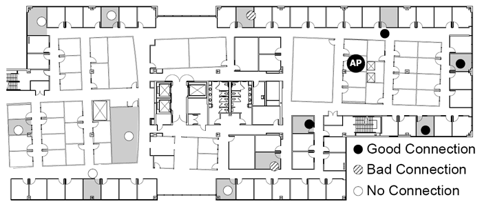
Figure 4: RF hole validation experiment. We attempted to connect to the shown AP from the shaded offices. The dots show the estimated client locations, and the classification of each location.
Finally, we also checked for RF holes on the operational WLAN in our building. The Connectivity Tracker did not find any clients that appeared to have difficultly connecting for more than 3 minutes, indicating that all areas of our floor have at least some WLAN coverage.
5.2 Deployment on a Operational Network
In this section, we demonstrate the utility of our system by using it to monitor the corporate WLAN on our floor. We present results generated by both the Client Performance Tracker and the Connectivity Tracker. Unless mentioned otherwise, the results described in this section are calculated over a period of one work-week; Monday, October 2nd through Friday, October 6th, 2006. We only report activity between 8am and 8pm each day, since there is very little traffic on the network outside of these hours. There was one 23 minute period of down-time on October 3rd due to a database misconfiguration.
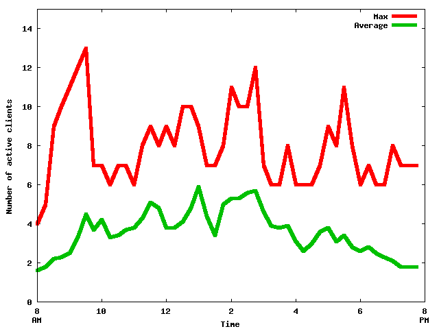
Figure 5:
Number of active clients per AP (15 minute interval)
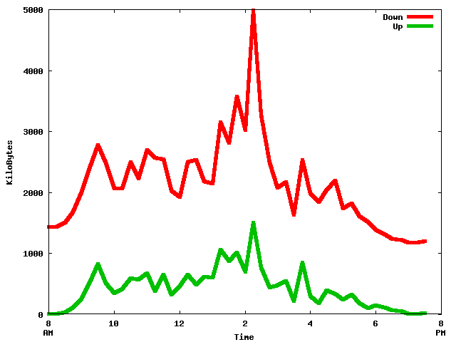
Figure 6:
UpLink and DownLink traffic per AP (15 minute interval)

Figure 7:
Distance between clients and the APs they attempt to associate with.

Figure 8:
Distance between APs and clients, when the session lasts longer than 60 seconds.
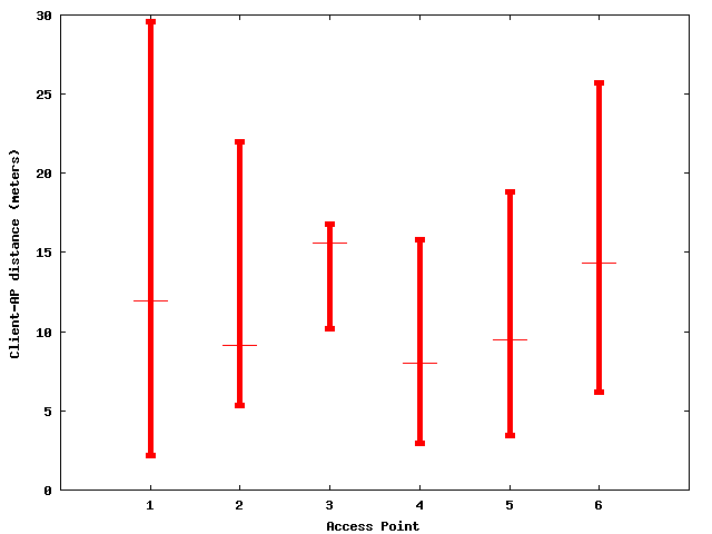
Figure 9:
Distance between active clients and APs: per-AP statistics ($10^{th}$ percentile, median and $90^{th}$ percentile).
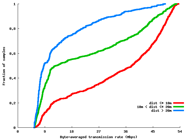
Figure 10:
Impact of distance between clients and APs on transmission rate of downlink traffic. (G clients only)
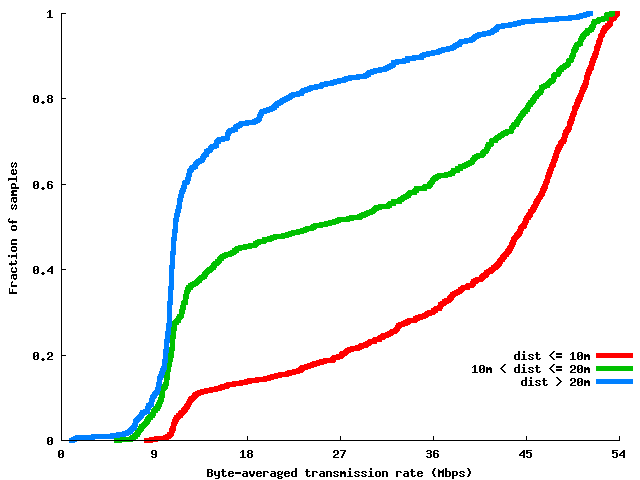
Figure 11:
Impact of distance between clients and APs on transmission rate of uplink traffic. (G clients only)
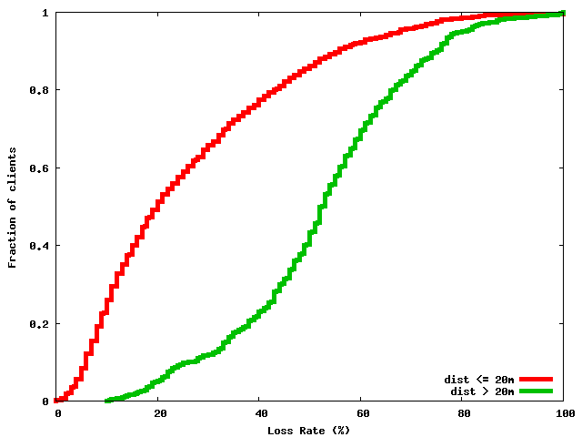
Figure 12:
Impact of distance between clients and APs on loss rate of downlink traffic.
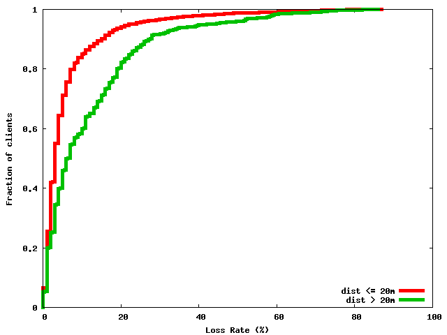
Figure 13:
Impact of distance between clients and APs on loss rate of upink traffic.
Because our building has four floors and our testbed is only deployed on one of them, we need to filter out clients who are located on other floors of our building. This is because we cannot report accurate locations for those clients, and because we cannot overhear any of their high data-rate transmissions. We performed experiments where we carried a laptop to the floors above and below our own, and we devised the following threshold based on those experiments: we consider a client to be located on our floor during a particular 15 minute interval if at least four AirMonitors overhear that client, and at least one of them reports a mean RSSI for transmissions from that client of at least -75 dBm.
Figures 5 and 6 provide a high-level view of the amount of activity on our WLAN. Figure 5 shows both the average and the maximum number of active clients on a per-AP basis for the six APs on our floor. The averages are calculated over 15 minute intervals, and “active” simply means that the client exchanged at least one frame with the AP. The number of clients associated with an AP can be as high as 12, although the average is lower. Figure 6
shows the average
uplink and downlink traffic (in kilobytes), measured over 15 minute
intervals. As expected, downlink traffic volume is substantially higher
than the uplink traffic volume.
Next, we look at client association patterns. Figure 7 shows the CDF of the distance between clients and the APs they attempt to associate with. Not all these association attempts are successful. However, it is interesting to see 40% of the clients attempt to associate with an AP that is over 20 meters away. This is surprising because the average distance to the nearest AP from any location on our floor is only 10.4 meters. While some of this discrepancy may be due to RF propagation effects, we believe that poor AP selection policies implemented in certain Wi-Fi drivers also play a role. While clients do attempt to associate with far-away APs, they generally do not stay associated with them for long. In Figure 8 we look at the connections that lasted for more than 60 seconds. We see that when a client is further than 20 meters from an AP, the probability that it will have a long-lived connection with that AP is small.
We also use client association behavior to evaluate the effectiveness of the AP placement on our floor. In Figure 9, we take a closer look at client distance from the perspective of the 6 APs on our floor. We find that for AP 3, the median distance of associated clients is larger than that of the other APs, and 90% of the clients that associate with this AP are more than 15 meters away. This is due to poor AP placement. This AP is supposed to serve the south end of our building, yet due to the presence of a large lab facility the offices at the far end of the building are too far away from this AP (and they are even further away from all other APs).
We also study the impact of client location on connection quality. We use two metrics to evaluate connection quality: byte-averaged transmission rate, and packet loss rate. For this evaluation, we only consider those clients that transmit at least 50 Data frames on either the uplink or the downlink.
Figures 10 and 11 show the impact of the distance between clients and APs on both uplink and downlink transmission rates. For these two graphs we only considered clients that were operating in 802.11g mode. The filtering is necessary because the maximum transmission rate for 802.11b is only 11 Mbps. These graphs illustrate two interesting points. First, we see that the distance between clients and APs has a significant impact on both uplink and downlink transmission rates. When a client is more than 20 meters away from an AP, the median data rate on both the uplink and the downlink is less than 10 Mbps. We also see that for a given distance, the uplink rates are generally higher than the downlink rates. We believe that this is due to two reasons. First, we measured that the APs on our floor use lower transmission power levels than most client Wi-Fi cards, and this is likely done to minimize interference. Second, the chosen rate is heavily in
influenced by the frame loss rate, and as we will see
shortly, the downlink loss rates are noticeably higher than the uplink ones.
We also looked at similar graphs for clients that appear to operate only in 802.11b mode. The impact of distance on the transmission rate is much less pronounced for these clients. This is because the maximum transmission rate is capped at 11 Mbps, and the lowest data rates (1 and 2 Mbps) are rarely used even at moderate distances.
Next, we look at the impact of distance on frame loss rates. Figures 12 and 13 show the downlink and uplink loss rates, respectively. We see that downlink loss rates are significantly higher than uplink loss rates. The median downlink loss rate for clients within 20 meters of the AP is 20%, while the median uplink loss rate is only 3%. Mahajan et. al. have reported comparable results in [26]. Furthermore, distance seems to have a much bigger impact on downlink loss rates than it has on uplink loss rates. The median downlink loss rate for clients that are more than 20 meters away from APs is almost 50%. Note that this is the MAC-layer frame loss rate. A 50% MAC layer loss rate, with 4 retransmissions which is typical for most 802.11 devices, would translate into a 6.25% loss rate at the network layer if losses were independent.
The high downlink loss rate may be the result of aggressive rate adaptation algorithms on the AP. As mentioned earlier, our APs transmit at lower power levels than most clients. An aggressive rate adaptation algorithm can cause a high frame loss rate at low transmit power. We investigated in detail those cases when the reported downlink loss rate was higher than 80%. In some of these cases none of the AirMonitors heard any of the ACK packets sent by the client, resulting in incorrect loss estimation, and the total number of frames transmitted was small. These cases account for less than 2% of the samples.
We also considered whether there are any regions on our floor where clients see consistently poor performance. We divided the area of our floor into 14 by 16 meter rectangles. We looked at the median loss rate and the median transmission rate of clients who were located in each regions. One area stood out as worse than the others, and is highlighted in Figure 14. The median downlink loss rate for clients in this area was 49%, which is substantially higher compared to clients in other regions. In addition, the median byte-averaged downlink transmission rates for clients in this area is only 7.3 Mbps. We also noticed that many clients in this area tend to associate with multiple APs, some on other floors. The circles in Figure 14 indicate locations from which the clients connected to at least 5 access points. In most other regions, the clients tend to associate with one or two APs. This indicates that poor AP placement is one potential cause of clients’ poor performance in this area.

Figure 14:
Region of poor performance. The circles indicate locations
where clients connected to at least 5 APs.
5.3 Effects of Density
We investigate the effects of AirMonitor density on our results by randomly selecting subsets of our 59 AirMonitors and eliminating the data collected by those AirMonitors from our analysis. We then recalculate the graphs shown in the previous section for three different densities: 25%, 50%, and 75%. Reducing the number of AirMonitors reduces the amount of traffic observed, and also reduces the accuracy of the location results. At 25% density, the total amount of traffic observed during the entire one week period is reduced to 78% of the original total, and at 50% density it is reduced to 95% of the original. We believe that many of the frames that are lost in the lower density configurations are those frames sent at higher transmission rates, and we are currently investigating this further.
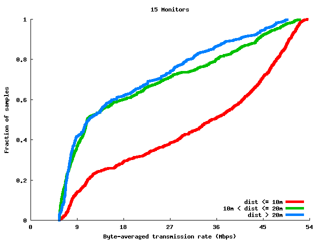
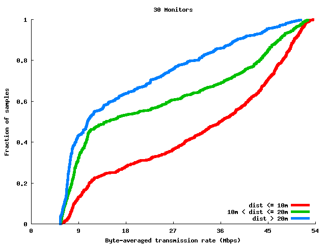
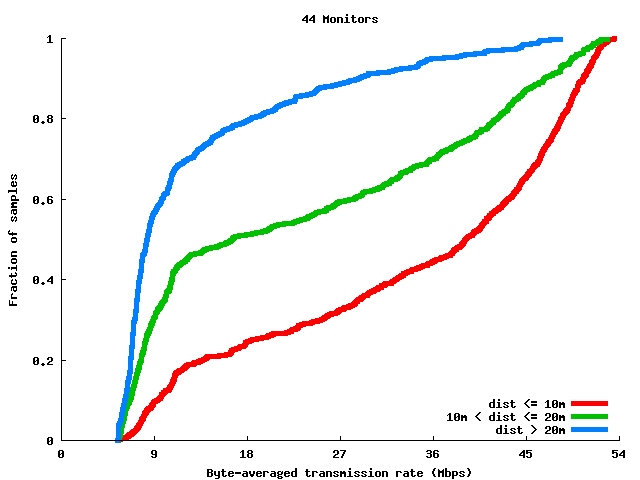
Figure 15:
Each figure shows the impact of the distance between clients and APs on downlink transmission rates. The three figures are calculated using AirMonitor densities of 25\%, 50\%, and 75\%, respectively.
For many of the performance statistics, we see qualitative differences in the results at densities of 25% and 50%, whereas the 75% density results tend to look quite similar to the 100% results. For example, in Figure 15, the three side-by-side graphs show the relationship between downlink transmission rates and the distance between clients and the APs to which they are associated. The leftmost graph shows the results for 25% AirMonitor density, the middle graph shows the results for 50% density, and right-most graph shows the 75% results. For comparison, the 100% density results are shown in the previous section in Figure 10.
6 Discussion
In this section, we discuss various issues related to the performance and effectiveness of our system.
- Our system determines the locations of the AirMonitors by guessing the primary user of the machine, and then reading the building map.
We repeat this process periodically to ensure accuracy of the AirMonitor locations.
If a machine is moved without its location being updated, the client locations that relied on observations from the moved AirMonitor may be in error. So
far, we have not had any problems with unannounced machine moves. We note that we can automatically detect when a machine is moved far away from its
original location. Each Air-Monitor is aware of its neighbors, and if the neighbor set changes significantly, the system administrator can be
notified. However, if the AirMonitor is moved only a short distance (say to the next office), we may not be able to automatically detect such a
move. In such cases, the error introduced in the estimated client locations is also likely to be small.
- We have not studied the accuracy of our location system in settings other than our office floor. It is likely that the
accuracy of the location system, and specifically, that of the Centroid algorithm, is helped by the fact that our offices have full-height
walls and solid wood doors. The radio signal fades rapidly in such an environment ensuring that only nearby AirMonitors hear a strong signal from a given
transmitter. In other settings (e.g. cubicles), many more AirMonitors may receive a strong signal from a given transmitter. This may degrade the accuracy
of the Centroid algorithm.
- Our system currently requires that each AirMonitor track the channel of nearest the AP. This strategy is appropriate for the management applications described in this paper, as clients in the region near an AP are also likely to associate that AP, and therefore operate on the same channel as our AirMonitors. Other channel assignment strategies may be appropriate for other applications. For example, for wireless security applications, it is desirable to monitor as much of the spectrum as possible in each area. This can be accomplished by having each AirMonitor randomly cycle through all channels, spending some time on each. We are also considering signal-strength based channel assignment.
- Because scalability is an important design goal, we briefly summarize measurements of our system’s scalability. During the full work week of operation, the size of all our database tables grew by just under 10 GB. Each AirMonitor generated less than 11 Kbps of traffic on the wired network submitting summaries to the database. We monitored the additional CPU load we placed on the Air-Monitors, and this load rarely exceeds 3%.
-
Both the loss rate and the transmission rate statistics
calculated by the Client Performance Tracker are estimates. For transmission rates, AirMonitors are less likely to overhear high transmission
rate frames, so it is likely that we are underestimating the true rates. We may overestimate loss rates if no AirMonitor overhears many of the Data packets
sent without the retry bit set. However, the results of our validation experiment in Table 2 give us confidence that this is unlikely.
7 Related work
Location Estimation: Many researchers have built systems for location estimation in WiFi networks. RADAR [7] uses pattern matching of received signal strength at a client from various landmarks, such as APs, to locate a Wi-Fi client. Further refinements of the idea appear in several subsequent papers [23, 22, 30, 10, 17]. These schemes include a manual profiling phase, which requires the network operator to collect RF fingerprints from a large number of locations. Many of these schemes are designed to allow WiFi clients to locate themselves not for the system to determine where the client is. We note that some of the techniques described in these papers can be used to enhance the accuracy of our system as well.
ActiveCampus [9] uses a hill-climbing algorithm to approximate the location of a mobile user using samples from multiple APs. The accuracy can be further enhanced by using feedback from mobile users.
The Placelab project [24] incorporates a self-mapping system that requires knowledge of only a few anchor nodes. This system is geared towards outdoor environments and the average location error is 31 meters.
Location estimation has also been studied for wireless sensor networks. Systems like MoteTrack [25] are designed for emergency management environments, and require extensive prior manual profiling. Sextant [16] uses a small number of landmark nodes to determine the region of a sensor node. It works by formulating geographic constraints on the location of the node. A key idea behind Sextant is to use information about which nodes can not hear each other. In our system, we can not be certain about the transmit power of the clients. Therefore we can not directly use Sextant’s model.
Location systems that use non-RF technologies such as ultrasound [29] are outside the scope of this work.
Research wireless network monitoring systems: Several researchers have studied mobility and traffic patterns in enterprise wireless networks. In [8], the authors characterize wireless traffic and user mobility in a large corporate environment using SNMP traces. They can not directly observe either user location or phenomena such as MAC-layer retransmissions. In [21, 18], the authors study traffic and usage patterns in an academic wireless network. In [20], the authors study usage patterns of WLAN at at IETF meeting. In these studies, the user location is characterized by the AP that the users are associated with. Our results show that users sometimes associate with APs that are far away.
Jigsaw [12] is a WLAN monitoring system that uses multiple monitors and trace combining to generate a comprehensive view of network events. There are two key differences between Jigsaw and our system. First, Jigsaw does not include a location engine and hence when it is used to detect performance problems it cannot provide specific information about the location(s) of the client(s) experiencing those problems. Second, Jigsaw is architecturally is very different from our system. Jigsaw uses dedicated, custom-built, multi-radio monitoring nodes whereas we add off-the-shelf USB wireless adapters to end-user desktops. Jigsaw generates full packet traces at every monitoring node and performs a centralized merge of these traces, whereas our monitors generate application-specific traffic summaries, and we attempt to select the “best” monitor for hearing a particular communication to avoid having to merge observations from multiple monitors. With full packet traces, Jigsaw can provide a detailed look at low-level network effects such as interference, that DAIR can only guess at.
In [15], the authors describe a simple packet capture utility and how they used it for intrusion detection. WIT [26] is a toolkit for analyzing the MAC-level behavior of WLANs using traces captured from multiple vantage points. The toolkit does not include a location estimation tool. We have discussed the relationship between WIT and our approach throughout the paper.
In [4], the authors present a system for diagnosing faults in Wi-Fi networks. They study some of the same problems that we do, and their techniques for locating disconnected clients are somewhat similar to ours. However, their system is based entirely on observations made by mobile clients. It requires installation of special software on clients. Furthermore, the accuracy of their location system is significantly worse than ours: they report a median error of 9.7 meters.
Commercial wireless network monitoring systems:
Currently, a few commercial systems are available for wireless network monitoring and diagnosis. Many of these systems focus on security issues such as detecting rogue APs, which was the subject of our previous paper [5].
Unlike research systems, only a few selective details are publicly available about the performance of commercial systems. Below, we present a summary comparison of DAIR with two commercial monitoring systems, using the claims they make in their marketing literature and white papers available on their websites.
AirTight Networks [2] sells a system called Spectra-Guard, which has many features similar to DAIR. Spectra-guard, however, requires the use of special sensor nodes that have to be manually placed in various places within the area to be monitored. It also requires special software to be installed on the clients. The system is focused on detecting threats such as rogue access points. Spectra-guard also provides RF coverage maps and some performance diagnostics, although the details are not available in the published data sheets. Spectraguard includes a location subsystem. However, details about how it works, and what accuracy it provides are unavailable.
AirDefense [1] also sells a system for monitoring of corporate wireless networks. Like SpectraGuard, this product also focuses on wireless security problems. It also requires use of special wireless sensors, and installation of special software on end systems. The key differentiating feature of this product is called “RF Rewind”. The sensors collect upto 270 measurements per wireless device per minute. This data can be later used for forensic investigations. The product includes some location determination features, although the details are not publicly available. It is not clear what performance diagnostic information is provided by AirDefense.
8 Conclusion
We have built a scalable, and easy-to-deploy WLAN management system that incorporates a self-configuring location engine. Using our system, we monitored an operational WLAN network. Our results show the importance of knowing the locations of WLAN clients in understanding their performance. Therefore, we have demonstrated the need for a location estimation engine to be an integral part of any WLAN management system. We have also demonstrated that by using a dense deployment of wireless sensors, one can use simple algorithms to estimate client location and performance. Finally, we showed that a dense deployment of wireless monitors can be achieved in a cost-effective manner using the DAIR platform.
Although the focus of this paper has been on using location to improve the performance and reliability of WLANs, the location engine we have built is also directly applicable to the wireless security management applications that were the focus of our previous DAIR paper [5].
Acknowledgments
We would like to thank Victor Bahl, Ratul Mahajan, John Dunagan, Krishna Gummadi and the anonymous reviewers for their helpful comments.
References
[1] AirDefense: Wireless LAN Security. https://airdefense.net.
[2] AirTight Netwoks. https://airtightnetworks.net.
[3] Aruba Networks. https://www.arubanetworks.com.
[4] A. Adya, P. Bahl, R. Chandra, and L. Qiu. Architecture and techniques for diagnosing faults in IEEE 802.11 infrastructure networks. In MOBICOM, 2004.
[5] P. Bahl, R. Chandra, J. Padhye, L. Ravindranath, M. Singh, A. Wolman, and B. Zill. Enhancing the security of corporate wi-fi networks using DAIR. In MobiSys, 2006.
[6] P. Bahl, J. Padhye, L. Ravindranath, M. Singh, A. Wolman, and B. Zill. DAIR: A framework for managing enterprise wireless networks using desktop infrastructure. In HotNets, 2005.
[7] P. Bahl and V. N. Padmanabhan. RADAR: An in-building rf-based user location and tracking system. In INFOCOM, 2000.
[8] M. Balazinska and P. Castro. Characterizing mobility and network usage in a corporate wireless local-area network. In MobiSys, 2003.
[9] E. Bhasker, S. W. Brown, and W. G. Griswold. Employing user feedback for fast, accurate, low-maintenance geolocationing. In IEEE Percom, 2004.
[10] P. Castro, P. Chiu, T. Kremenek, and R. Muntz. A probabilistic room location service for wireless networked environments. In UBICOMP, 2001.
[11] R. Chandra, J. Padhye, A. Wolman, and B.Zill. A Location-Based Management System for Enterprise Wireless LANs. Microsoft Research Technical Report MSR-TR-2007-16. February 2007.
[12] Y.-C. Cheng, J. Bellardo, P. Benko, A. Snoeren, G. Voelker, and S. Savage. Jigsaw: Solving the puzzle of enterprise 802.11 analysis. In SIGCOMM, 2006.
[13] F. Dabek, R. Cox, F. Kaashoek, and R. Morris. Vivaldi: A decentralized network coordinate system. In SIGCOMM, 2004.
[14] J. R. Douceur and W. J. Bolosky. Progress-based regulation of low-importance processes. In SOSP, 1999.
[15] S. Felis, J. Quittek, and L. Eggert. Measurement based wireless LAN troubleshooting. In WinMee, 2005.
[16] S. Guha, R. Murty, and E. G. Sirer. Sextant: A unified node and event localization framework using non-convex constraints. In MobiHoc, 2005.
[17] A. Haeberlen, E. Flannery, A. M. Ladd, A. Rudys, D. S. Wallach, and L. E. Kavraki. Practical robust localization over large-scale 802.11 wireless networks. In MOBICOM, 2004.
[18] T. Henderson, D. Kotz, and I. Abyzov. The changing usage of a mature campus-wide wireless network. In MOBICOM, 2004.
[19] IEEE802.11b/D3.0. Wireless LAN Medium Access Control(MAC) and Physical (PHY) Layer Specification: High Speed Physical Layer Extensions in the 2.4 GHz Band, 1999.
[20] A. Jardosh, K. Ramachandran, K. C. Almeroth, and E. M. Belding-Royer. Understanding congestion in IEEE 802.11b wireless networks. In IMC, 2005.
[21] D. Kotz and K. Essien. Analysis of a campus-wide wireless network. In MOBICOM, 2002.
[22] J. Krumm and E. Horvitz. Locadio: Inferring motion and location from WiFi signal strengths. In Mobiquitous, 2004.
[23] A. M. Ladd, K. E. Bekris, A. Rudys, G. Marceau, L. E. Kavraki, and D. S. Wallach. Robotics-based location sensing using wireless ethernet. In MOBICOM, 2002.
[24] A. LaMarca, J. Hightower, I. Smith, and S. Consolvo. Self-mapping in 802.11 location systems. In Ubicomp, 2005.
[25] K. Lorincz and M. Welsh. Motetrack: A robust, decentralized approach to RF-based location tracking. In LoCA, 2005.
[26] R. Mahajan, M. Rodrig, D. Wetherall, and J. Zahorjan. Analyzing MAC-level behavior of wireless networks in the wild. In SIGCOMM, 2006.
[27] Microsoft Active Directory. https://www.microsoft.com/windows/
server2003/technologies/directory/activedirectory/.
[28] D. Mills. Network time protocol (version 3) specification, implementation and analysis. RFC 1305, March 1992.
[29] N. B. Priyantha, A. Miu, and H. Balakrishnan. The Cricket location-support system. In MOBICOM, 2001.
[30] M. A. Youssef, A. Agrawala, and A. U. Shankar. WLAN location determination via clustering and probability distributions. In IEEE Percom, 2003.
|