Sparse Approximations for High
Fidelity
Compression of Network Traffic Data
William Aiello  |
Anna Gilbert |
Brian Rexroad |
Vyas Sekar  |
| University of British
Columbia |
University of Michigan |
AT & T Labs |
Carnegie Mellon
University |
| aiello@cs.ubc.ca |
annacg@umich.edu |
brexroad@att.com |
vyass@cs.cmu.edu |
An important component of traffic analysis and network monitoring is
the ability to correlate events across multiple data streams, from
different sources and from different time periods. Storing such a large
amount of data for visualizing traffic trends and for building
prediction models of ``normal'' network traffic represents a great
challenge because the data sets are enormous. In this paper we present
the application and analysis of signal processing techniques for
effective practical compression of network traffic data. We propose to
use a
sparse approximation of the network traffic data over a
rich collection of natural building blocks, with several natural
dictionaries drawn from the networking community's experience with
traffic data. We observe that with such natural dictionaries, high
fidelity compression of the original traffic data can be achieved such
that even with a compression ratio of around 1:6, the compression error,
in terms of the energy of the original signal lost, is less than 1%. We
also observe that the sparse representations are stable over time, and
that the stable components correspond to well-defined periodicities in
network traffic.
Traffic monitoring is not a simple task. Network operators have to deal
with large volumes of data, and need to identify and respond to network
incidents in real-time. The task is complicated even further by the fact
that monitoring needs to be done on multiple dimensions and timescales.
It is evident that network operators wish to observe traffic at finer
granularities across different dimensions for a multitude of reasons
that include: 1. real-time detection and response to network failures
and isolating errant network segments, 2. real-time detection of network
attacks such as DDoS and worms, and installation of filters to protect
network entities, and 3. finer resolution root-cause analysis of the
incidents and automated/semi-automated drill down of the incident. To
meet these requirements, we must be able to generate and store traffic
data on multiple resolution scales in space (network prefixes and
physical network entities such as links, routers), and in time (storing
the traffic aggregates at multiple time resolutions). Such requirements
naturally translate into increased operational costs due to the
increased storage requirement. We often transport large portions of the
historical data across a network to individual operators, import pieces
of data into statistical analysis and visualization software for
modeling purposes, and index and run queries against various historical
databases for data drill down. Thus the management overhead involved in
handling such large data sets, and the computational overhead in
accessing and processing the large volumes of historical data also
increases. We must reduce the storage size of the data, not only for
efficient management of historical traffic data, but also to accommodate
fine data resolution across space and time. The compression techniques
we investigate are ``lossy'' compression methods. For most network
monitoring applications that utilize historical traffic data, it often
suffices to capture salient features of the underlying traffic. We can
thus afford some error by ignoring the low-energy stochastic components
of the signal, and gain better compression using lossy compression
techniques (as opposed to lossless compression methods such as
gzip [
11] which
reduce the storage size of the data only and do not reduce the size of
the input to monitoring applications). The overall goal of such
compression techniques is to obtain high fidelity (i.e. low error)
representations with as little storage as possible. In particular, we
use a compression method called sparse representation over redundant
dictionaries. A visual inspection of aggregated network traffic for many
high volume ports reveals three components. First, there is a natural
diurnal variation for many ports and/or other periodic variations as
well. Second, there are spikes, dips, and other components of the
traffic that appear to be the result of non-periodic events or
processes. Finally, the traffic appears to be stochastic over small time
scales with variance much smaller than the periodic variations for high
volume ports. Representing a signal with all three components using a
single orthonormal basis, such as a Fourier basis or a wavelet
representation is not likely to yield good compression: a basis that
represents periodic signals well will not represent non-periodic signals
efficiently and vice versa. The methods presented in this paper allow
us to use two or more orthonormal bases
simultaneously. A set
of two or more orthonormal bases is called a redundant dictionary.
Hence, with an appropriate set of orthonormal bases as the redundant
dictionary, the periodic and the significant non-periodic portions of
the traffic time series can both be represented efficiently within the
same framework. Sparse representation or approximation over redundant
dictionaries does not make assumptions about the underlying
distributions in the traffic time series. As a result, sparse
approximation can guarantee high fidelity regardless of changes in the
underlying distributions. In addition, there are highly efficient,
provably correct algorithms for solving sparse approximation problems.
These algorithms scale with the data and can be easily adapted to
multiple sources of data. They are greedy algorithms, known as matching
or orthogonal matching pursuit. The primary contribution of this paper
is a rigorous investigation of the method of sparse representation over
redundant dictionaries for the compression of network time series data.
We propose and evaluate several redundant dictionaries that are
naturally suited for traffic time series data. We conclude that these
methods achieve significant compression with very high fidelity across a
wide spectrum of traffic data. In addition, we also observe that the
sparse representations are stable, not only in terms of their selection
in the sparse representation over time but also in terms of the
individual amplitudes in the representation. These stable components
correspond to well-defined periodicities in network traffic, and capture
the natural structure of traffic time series data. To the best of our
knowledge, this is the first thorough application of sparse
representations for compressing network traffic data. We discuss related
work in Section
2,
and present a overall motivation for compression in Section
3. In
Section
4 we
describe in more detail the framework of matching (greedy) pursuit over
redundant dictionaries. Section
5 describes our
traffic data set, derived from a large Internet provider. We evaluate
the efficacy of our compression techniques in Section
6. Section
7 presents
some network traffic monitoring applications that demonstrate the
utility of the compression methods we used. Section
8 discusses the
scope for improving the compression, before we conclude in Section
9.
2 Related Work
Statisticians concern themselves with subset selection in
regression [
13]
and electrical engineers use sparse representations for the compression
and analysis of audio, image, and video signals (see [
12,
6,
4] for several
example references). Lakhina, et al. [
10,
9] examine the
structure of network traffic using Principal Component Analysis (PCA).
The observations in our work provide similar insight into the structure
of network traffic. There are two compelling reasons for using sparse
approximations over redundant dictionaries, as opposed to PCA alone, for
obtaining similar fidelity-compression tradeoffs. First, the description
length for sparse approximation is much shorter than for PCA, since the
principal vectors require substantially more space to represent than
simple indices into a dictionary. Second, PCA like techniques may
capture and identify the (predominant) structure across all
measurements, but may not be adequate for representing subtle
characteristics on individual traffic aggregates. Barford, et al. [
1] use pseudo-spline
wavelets as the basis wavelet to analyze the time localized normalized
variance of the high frequency component to identify signal anomalies.
The primary difference is our application of signal processing
techniques for compressing network traffic data, as opposed to using
signal decomposition techniques for isolating anomalies in time series
data. There are several methods for data reduction for generating
compact traffic summaries for specific real-time applications. Sketch
based methods [
8]
have been used for anomaly detection on traffic data, while Estan et
al. [
3]
discuss methods for performing multi-dimensional analysis of network
traffic data. While such approaches are appealing for real-time traffic
analysis with low CPU and memory requirements, they do not address the
problems of dealing with large volumes of historical data that arise in
network operations. A third, important method of reducing data is
sampling [
2]
the raw data before storing historical information. However, in order
for the sampled data to be an accurate reflection of the raw data, one
must make assumptions regarding the underlying traffic distributions.
3 Compression
It is easy to (falsely) argue that compression techniques have
considerably less relevance when the current cost of (secondary) storage
is less than $1 per GB. Large operational networks indeed have the
unenviable task of managing many terabytes of measurement data on an
ongoing basis, with multiple data streams coming from different routers,
customer links, and measurement probes. While it may indeed be feasible
to collect, store, and manage such a large volume of data for small
periods of time (e.g. for the last few days), the real problem is in
managing large volumes of historical data. Having access to historical
data is a crucial part of a network operator's diagnostic toolkit. The
historical datasets are typically used for building prediction models
for anomaly detection, and also for building visual diagnostic aids for
network operators. The storage requirement increases not only because of
the need for access to large volumes of historical traffic data, but
also the pressing need for storing such historical data across different
spatial and temporal resolutions, as reference models for fine-grained
online analysis. It may be possible to specify compression and
summarization methods for reducing the storage requirement for specific
traffic monitoring applications that use historical data. However, there
is a definite need for historical reference data to be stored at fine
spatial and temporal resolutions for a wide variety of applications, and
it is often difficult to ascertain the set of applications and
diagnostic techniques that would use these datasets ahead of time. The
compression techniques discussed in this paper have the desirable
property that they operate in an application-agnostic setting, without
making significant assumptions regarding the underlying traffic
distributions. Since many traffic monitoring applications can tolerate a
small amount of error in the stored values, lossy compression
techniques that can guarantee a high fidelity representation with small
storage overhead are ideally suited for our requirements. We find that
our techniques provide very accurate compressed representations so that
there is only a negligible loss of accuracy across a wide spectrum of
traffic monitoring applications. The basic idea behind the compression
techniques used in this paper is to obtain a sparse representation of
the given time series signal using different orthonormal and redundant
bases. While a perfect lossless representation can be obtained by
keeping all the coefficients of the representation (e.g. using all
Fourier or wavelet coefficients), we can obtain a compressed (albeit
lossy) representation by only storing the high energy coefficients,
that capture a substantial part of the original time series signal.
Suppose we have a given time series signal of length

. For
example, in our data set consisting of hourly aggregates of traffic
volumes, N=168 over a week, for a single traffic metric of interest. We
can obtain a lossless representation by using up a total storage of

bits, where

represents the
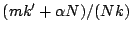
cost of storing each data point. Alternatively, we can obtain a sparse
representation using

coefficients using a total
storage space of

bits, where the term

represents the length of the dictionary used for
compression, and

represents the cost of storing the
amplitude associated with each coefficient. The
term represents the cost of storing the list of
selected indices as a bit-vector of length equal to the size of the
dictionary. The length of the dictionary
is
equal to

, with the value

being one for an orthonormal basis (e.g., Fourier, Wavelet, Spike) or
equal to two in the case of a redundant dictionary consisting of Fourier
and Spike waveforms. The effective compression ratio is thus
. Assuming

(the cost of storing the raw and compressed
coefficients are similar) and

(the values in consideration are large integers
or floats), the effective compression (even with this naive encoding) is
approximately equal to
 1
1. The primary
focus of this paper is not to come up with an optimal encoding scheme
for storing the
coefficients to extract the greatest
per-bit compression. Rather we wish to explore the spectrum of signal
compression techniques, using different natural waveforms as
dictionaries for achieving a reasonable error-compression tradeoff. A
natural error metric for lossy compression techniques in signal
processing is the energy of the residual, which is the vector difference
between the original signal and the compressed representation. Let

be the original signal and

represent the
compressed representation of
. The signal

represents the residual signal. We use the
following relative error metric

where

represents the

(Euclidean)
norm of a vector. The error metric represents the fraction of the
energy in the original signal that is not captured in the compressed
model. For example, a relative error of 0.01 implies that the energy of
the residual signal (not captured by the compressed representation) is
only 1% of the energy of the original signal. Our results indicate that
we can achieve high fidelity compression for more than 90% of all
traffic aggregates, with a relative error of less than 0.01 using only

coefficients, for the hourly aggregates with

. Since a m-coefficient representation of the signal
implies a compression ratio of roughly
, with
, a 30-coefficient representation corresponds to a
compression ratio of roughly 1:6. Consider the following scenario. An
operator wishes to have access to finer resolution historical reference
data collected on a per application port basis (refer Section
5 for a detailed
description of the datasets used in this paper). Suppose the operator
wants to improve the temporal granularity by going from hourly
aggregates to 10 minute aggregates. The new storage requirement is a
non-negligible
, where

represents the
current storage requirement (roughly 1GB of raw data per router per
week). Using the compression techniques presented in this paper, by
finding small number of dictionary components to represent the time
series data, the operator can easily offset this increased storage cost.
Further, we observe (refer Section
8.2) that
moving to finer temporal granularities does not actually incur
substantially higher storage cost. For example we find that the same
fidelity of compression (at most 1% error) can be obtained for
time-series data at fine time granularity (aggregated over five minute
intervals) by using a similar number of coefficients as those used for
data at coarser time granularities (hourly aggregates). Thus by using
our compression techniques operators may in fact be able to
substantially cut down storage costs, or alternatively use the storage
``gained'' for improving spatial granularities (collecting data from
more routers, customers, prefixes, etc). In the next section, we present
a brief overview on the use of redundant dictionaries for compression,
and present a greedy algorithm for finding a sparse representation over
a redundant dictionary.
4 Sparse Representations over Redundant Dictionaries
One mathematically rigorous method of compression is that of sparse
approximation. Sparse approximation problems arise in a host of
scientific, mathematical, and engineering settings and find greatest
practical application in image, audio, and video compression [
12,
6,
4], to name a few.
While each application calls for a slightly different problem
formulation, the overall goal is to identify a good approximation
involving a few elementary signals--a
sparse approximation.
Sparse approximation problems have two characteristics. First, the
signal vector is approximated with a linear model of elementary
signals (drawn from a fixed collection of several orthonormal bases).
Second, there is a compromise between approximation error (usually
measured with Euclidean norm) and the number of elementary signals in
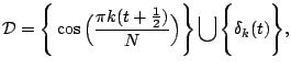
the linear combination. One example of a redundant dictionary for
signals of length
is the union
where
,
of the cosines and the spikes on
points. The
``spike'' function

is zero if

and is one
if

. Either basis of vectors is complete
enough to represent a time series of length
but it might take
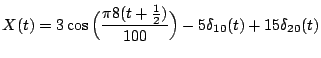
more vectors in one basis than the other to represent the signal. To
be concrete, let us take the signal
plotted in Figure
1(a).
Figure 1: The example signal and its discrete cosine transform (DCT).
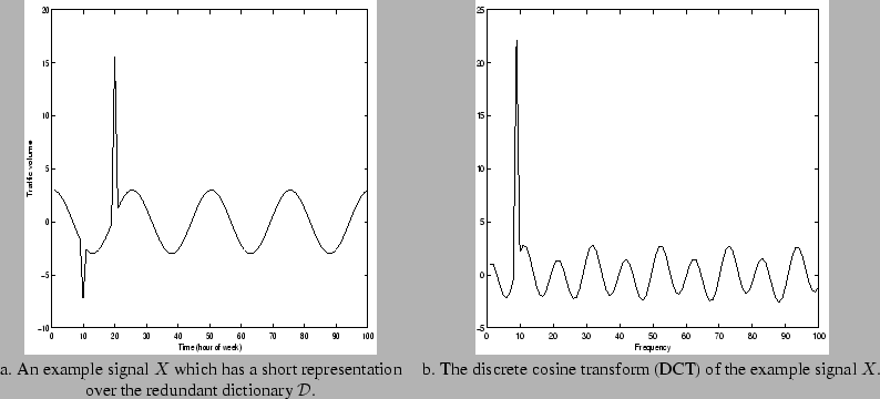 |
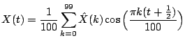
The spectrum of the discrete cosine transform (DCT) of
is
plotted in Figure
1(b). For this
example, all the coefficients are nonzero. That is, if we write
as a linear combination of vectors from the cosine basis, then all 100
of the coefficients

are nonzero. Also, if
we write

as a linear combination of spikes, then
we must use almost all 100 coefficients as the signal
is
nonzero in almost all 100 places. Contrast these two expansions for
with the expansion over the redundant dictionary

In this expansion there are only three nonzero coefficients, the
coefficient 3 attached to the cosine term and the two coefficients
associated with the two spikes present in the signal. Clearly, it is
more efficient to store three coefficients than all 100. With three
coefficients, we can reconstruct or decompress the signal exactly. For
more complicated signals, we can keep a few coefficients only and obtain
a good approximation to the signal with little storage. We obtain a
high fidelity (albeit lossy) compressed version of the signal. Observe
that because we used a dictionary which consists of simple, natural
building blocks (cosines and spikes), we need not store 100 values to
represent each vector in the dictionary. We do not have to write out
each cosine or spike waveform explicitly. Finding the optimal dictionary
for a given application is a difficult problem and good approximations
require domain specific heuristics. Our contribution is the
identification of a set of dictionaries that are well-suited for
compressing traffic time-series data, and in empirically justifying the
choice of such dictionaries. Prior work on understanding the
dimensionality of network traffic data using principal component
analysis [
10]
identifies three types of eigenflows: periodic, spikes, and noise. With
this intuition, we try different dictionaries drawn from three basic
waveforms: periodic functions (or complex exponentials), spikes, and
wavelets. Dictionaries that are comprised of these constituent signals
are descriptive enough to capture the main types of behavior but not so
large that the algorithms are unwieldy.
A greedy pursuit algorithm at each iteration makes the best local
improvement to the current approximation in hope of obtaining a good
overall solution. The primary algorithm is referred to as Orthogonal
Matching Pursuit (OMP), described in Algorithm
4.1. In each step
of the algorithm, the current best waveform is chosen from the
dictionary to approximate the residual signal. That waveform is then
subtracted from the residual and added to the approximation. The
algorithm then iterates on the residual. At the end of the pursuit
stage, the approximation consists of a linear combination of a small
number of basic waveforms. We fix some notation before describing the
algorithm. The dictionary
consists of

vectors

of length
each. We write
these vectors
as the rows in a matrix

and refer to this matrix as the dictionary matrix.
OMP is one of the fastest
2 provably correct algorithm for
sparse representation over redundant dictionaries, assuming that the
dictionary satisfies certain geometric constraints [
5] (roughly, the
vectors in the dictionary must be almost orthogonal to one another). The
algorithm is provably correct in that if the input signal consists of a
linear combination of exactly
vectors from the dictionary, the
algorithm finds those
vectors exactly. In addition, if
the signal is not an exact combination of
vectors but it
does have an optimal approximation using
vectors, then the
algorithm returns an
-term linear combination whose
approximation error to the input signal is within a constant factor of
the optimal approximation error. If we seek
vectors in our
representation, the running time of OMP is

.
Dictionaries which are unions of orthonormal bases (which meet the
geometric condition for the correctness of OMP), are of size

, so the running time for OMP with such dictionaries is

.
Note that if we had a single orthonormal basis as the dictionary
, the representation obtained using Algorithm
4.1 is exactly the
same as the projection onto the orthonormal basis. For example, if we
just had a Fourier basis, the coefficients obtained from a regular
Fourier transform would exactly match the coefficients obtained from the
matching pursuit procedure.
5 Data Description
The primary data set we have used for evaluating our methods consists
of traffic aggregates collected over a 20 week period (between January
and June 2004) at a large Tier-1 Internet provider's IP backbone
network. The dataset consists of traffic aggregates in terms of flow,
packet, and byte counts. The dimensions of interest over which the
aggregates are collected are:
- TCP Ports: Traffic to and from each of the 65535 TCP ports.
- UDP Ports: Traffic to and from each of the 65535 UDP ports.
- Aggregated Network Prefixes: Traffic to and from network prefixes
aggregated at a set of predefined network prefixes.
The traffic aggregates were generated from flow records using
traffic collection tools similar to Netflow [14], aggregated over
multiple links in the provider's Internet backbone. In this particular
data set, the traffic volume counts are reported on an hourly basis. For
example, for each TCP port the data set contains the total number of
flows, packets, and bytes on that port. The data set aggregates each
metric (i.e., flows, packets, and bytes) for both incoming (i.e.,
traffic with this port was the destination port) and outgoing traffic
(i.e., traffic with this port as the source port). Such per-port and
per-prefix aggregates are routinely collected at many large ISPs and
large enterprises for various traffic engineering and traffic analysis
applications.
It is useful to note that such data sets permit interesting traffic
analysis including observing trends in the traffic data, and detecting
and diagnosing anomalies in the network data. For many types of network
incidents of interest (outages, DoS and DDoS attacks, worms, viruses,
etc.) the dataset has sufficient spatial granularity to diagnose
anomalies. For example, the number of incoming flows into specific ports
can be an indication of malicious scanning activity or worm activity,
while the number of incoming flows into specific prefixes may be
indicative of flash-crowds or DoS attacks targeted at that prefix.
For the following discussions, we consider the data in week long
chunks, partly because a week appears to be the smallest unit within
which constituent components of the signal manifest themselves, and also
because a week is a convenient time unit from an operational viewpoint.
6 Results
In this section, we demonstrate how we can use sparse approximations to
compress traffic time series data. We look at the unidimensional
aggregates along each port/protocol pair and prefix as an independent
univariate signal. In the following sections, unless otherwise stated,
we work with the total number of incoming flows into a particular port.
We observe similar results with other traffic aggregates such as the
number of packets and the number of incoming bytes incoming on each
port, and for aggregated counts for the number of outgoing flows,
packets, bytes on each port--we do not present these results for
brevity. We present the results only for the TCP and UDP ports and note
that the compression results for aggregated address prefixes were
similar. Since an exhaustive discussion of each individual port would be
tedious, we identify 4 categories of ports, predominantly characterized
based on the applications that use these ports. For each of the
categories the following discussion presents results for a few canonical
examples.
- High volume, popular application ports (e.g., HTTP, SMTP, DNS).
- P2P ports (e.g., Kazaa, Gnutella, E-Donkey).
- Scan target ports (e.g., Port 135, Port 139) .
- Random low volume ports.
6.1 Fourier Dictionary
Our first attempt at selecting a suitable dictionary for compression
was to exploit the periodic structure of traffic time series data. A
well known fact, confirmed by several measurements [
9,
10,
15], is the fact that
network traffic when viewed at sufficient levels of aggregation exhibits
remarkably periodic properties, the strongest among them being the
distinct diurnal component. It is of interest to identify these using
frequency spectrum decomposition techniques (Fourier analysis). It is
conceivable that the data can be compressed using a few fundamental
frequencies, and the traffic is essentially a linear combination of
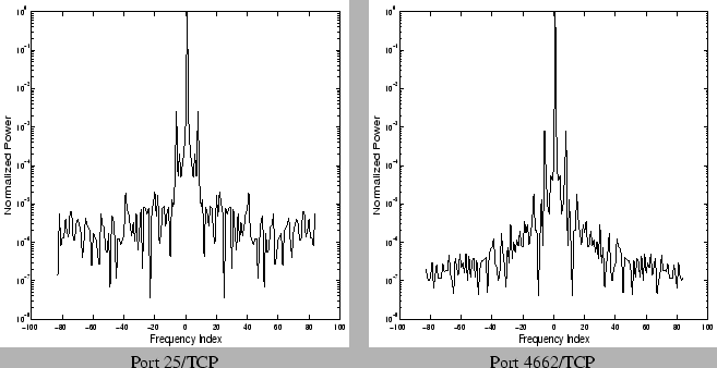
these harmonics with some noisy stochastic component. To understand the
intuition behind using the frequency spectrum as a source of compression
we show in Figure
2 the
power spectrum of two specific ports for a single week. In each case
the power spectrum amplitudes are normalized with respect to the maximum
amplitude frequency for that signal (usually the mean or

frequency component), and the y-axis is shown on a log-scale after
normalization. We observe that the power spectrum exhibits only a few
very high energy components. For example the central peak and the high
energy band around it corresponds to the mean (
)
frequency in the Fourier decomposition, while the slightly lesser peaks
symmetric around zero, and close to it correspond to the high energy
frequencies that have a wavelength corresponding to the duration of a
day.
Figure 2: Frequency power
spectrum of time-series of incoming flows on specific ports over a
single week
 |
We also show the how the normalized amplitude decreases when we sort
the frequency components in descending order of their amplitudes in
Figure
3.
We observe that there is indeed a sharp drop (the figures are in
log-scale on y-axis) in the energy of the frequency components after
20-30 components for the different signals considered.
Figure 3: Energy of the
frequencies sorted in descending order for specific ports
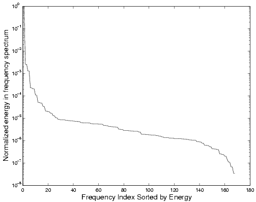
|
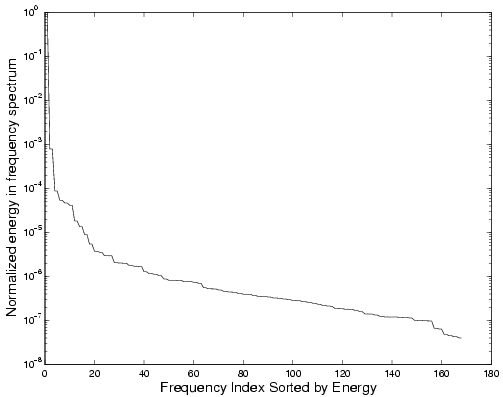
|
Port 25/TCP
|
Port 4662/TCP
|
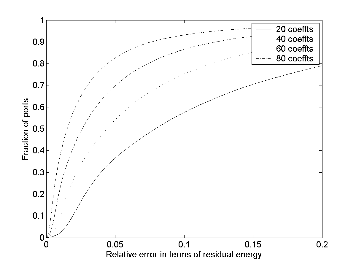
We observe that a small number of components do capture a significant
portion of the energy, which suggests a rather obvious compression
scheme. For each week-long time series, pick the
frequencies that have the highest energies in the power spectrum.
Figure
4
indicates that using 40 coefficients per week (around 40/168 = 25% of
the original signal size) coefficients yields a relative error of less
than 0.05 for more than 90% of all ports
3. A relative error
of 0.05 using our relative error metric indicates that around 95% of the
original signal energy was captured in the compressed form. We observe
in Figure
5
that the corresponding compressibility of UDP ports is slightly worse.
The reason is that the traffic volumes on UDP ports tend to exhibit far
lesser aggregation, in terms of absolute volumes and popularity of usage
of particular ports. Intuitively one expects that with higher volumes
and aggregation levels, the traffic would exhibit more periodic
structure, which explains the better compression for TCP ports as
opposed to UDP ports.
Figure 4: CDFs of relative
error for TCP ports (incoming flows) with Fourier dictionary
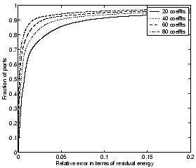 |
Figure 5: CDFs of relative
error for UDP ports (incoming flows) with Fourier dictionary
|
The Fourier basis is one simple orthonormal basis. There are a host
of other orthonormal bases which have been employed for compressing
different datasets. Wavelets have traditionally been used for
de-noising and compression in image and audio applications. The
effectiveness of a wavelet basis depends on the choice of the ``mother
wavelet'' function. However, identifying the best basis for representing
either a given signal or a class of signals is a hard problem, for
which only approximate answers exist using information-theoretic
measures [
17].
For our experiments we tried a variety of wavelet families including
the well studied Daubechies family of wavelets, and other derivatives
such as Symlets and Coiflets. Our observation is that the families of
wavelets we tested had poorer performance when compared with the
Fourier basis. Although an exhaustive discussion of choosing the ideal
wavelet family is beyond the scope of this paper, our experiments with a
host of wavelet families indicate that the traffic time-series cannot be
efficiently compressed using wavelets (as an orthonormal basis) alone.
Our choice of the Fourier dictionary was motivated by the observation
that the traffic time-series when viewed at a reasonable level of
aggregation possesses a significant periodic component. Therefore, using
Fourier basis functions as part of the redundant dictionary seems a
reasonable starting point. There are however, other interesting
incidents we wish to capture in the compressed representation.
Experience with traffic data indicates that interesting events with high
volume (and hence high signal energy) include possibly anomalous spikes,
traffic dips, and slightly prolonged high traffic incidents. Such
isolated incidents, localized in time, cannot be succinctly captured
using only a Fourier basis. Fortunately, these events can be modeled
either using spike functions appropriately placed at different time
indices, or using Haar wavelets (square waveforms) of different scales
and all translations. The fully-translational Haar wavelets at all
scales and all translations form a rich redundant dictionary of size

. By contrast, the orthonormal basis of Haar
wavelets is of size
and consists of the Haar wavelets
at all scales and only those translations which match the scale of the
wavelet. Table
1
compares a host of possible dictionaries on selected ports. Over the
entire spectrum of port types, we observe that specific bases are indeed
better suited than others for specific ports. For example, we observe
that for some high volume and P2P ports using a Fourier dictionary gives
better compression than using a wavelet or full-translation Haar
dictionary, while for some of the random and scan ports, the wavelet or
full-translation Haar dictionary give better compression. In some cases
(e.g. port 114) we also find that using spikes in the dictionary gives
the lowest compression error.
Table 1: Compression error with 30
coefficient representation for selected TCP ports (Legend: F = Fourier,
W = Ortho-normal db4 wavelets,
H = Fully-translational Haar wavelets, S = Spikes)
| Port
Type |
Port
Number |
Relative error with different
dictionaries |
| DF |
DW |
DS |
DH |
DF+S |
DF+H |
DF+H+S |
DH+S |
| High
Volume |
25 |
0.0005 |
0.0026 |
0.8446 |
0.0007 |
0.0004 |
0.0004 |
0.0004 |
0.0007 |
| 80 |
0.0052 |
0.0256 |
0.7704 |
0.0074 |
0.0052 |
0.0018 |
0.0018 |
0.0073
|
| P2P |
1214 |
0.0003 |
0.0036 |
0.0007 |
0.8410 |
0.0003 |
0.0001 |
0.0001 |
0.0007 |
| 6346 |
0.0009 |
0.0056 |
0.8193 |
0.0013 |
0.0009 |
0.0005 |
0.0005 |
0.0013
|
| Scan |
135 |
0.0016 |
0.0216 |
0.7746 |
0.0049 |
0.0015 |
0.0008 |
0.0008 |
0.0049 |
| 9898 |
0.0066 |
0.0143 |
0.7800 |
0.0036 |
0.0063 |
0.0032 |
0.0032 |
0.0036
|
| Random |
5190 |
0.0023 |
0.0280 |
0.7916 |
0.0040 |
0.0023 |
0.0010 |
0.0010 |
0.0039 |
| 114 |
0.5517 |
0.1704 |
0.0428 |
0.0218 |
0.0097 |
0.0218 |
0.0068 |
0.0068
|
Rather than try to optimize the basis selection for each specific port,
we wish to use redundant dictionaries that can best capture the
different components that can be observed across the entire spectrum of
ports. Hence we use redundant dictionaries composed of Fourier,
fully-translational Haar, and Spike waveforms and observe that we can
extract the best compression (in terms of number of coefficients
selected), across an entire family of traffic time series data. We
compare three possible redundant dictionaries: Fourier+ Haar wavelets
(referred to as

), Fourier + Spikes (referred to as

), and Fourier + Spikes + Haar wavelets (referred to
as

). Within each dictionary the error-compression
tradeoff is determined by the number of coefficients chosen (Recall that
a m-coefficient representation roughly corresponds to a compression
ratio of
). A fundamental property of the greedy
pursuit approach is that with every iteration the residual energy
decreases, and hence the error is a monotonically decreasing function of
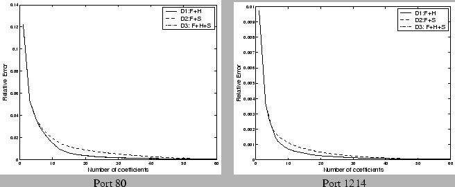
the number of modes chosen. We evaluate the error-compression tradeoffs
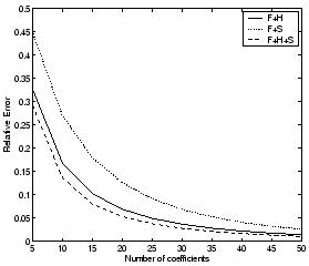
for these different dictionaries in Figures
6 and
7, where
we assume that we are constrained to use 30 coefficients (roughly
corresponding to using only one-sixth of the data points for each week).
We observe two main properties of using the redundant dictionary
approach. First, the compressibility is substantially enhanced by
expanding the dictionary to include either spikes or Haar wavelets, in
addition to the periodic Fourier components, i.e., using redundant
dictionaries yields better fidelity for the same storage cost as
compared to a single orthonormal basis. The second property we observe
with the particular choice of basis functions on the traffic data is a
monotonicity property - adding a richer basis set to the dictionary
helps the compressibility. For example the error-compression tradeoff
that results with
is never worse than either
or
. The compression does come
at a slightly higher computation cost, since the time to compress the
time series depends on the size of the dictionary used, as the
compression time scales in linearly with the number of vectors in the
dictionary (refer Section
4).
Figure 6: CDFs of relative
error for TCP ports (incoming flows) with 30 coefficients for different
dictionaries
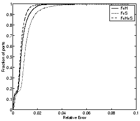 |
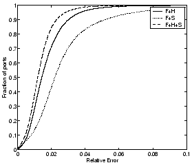
Figure 7: CDFs of relative
error for UDP ports (incoming flows) with 30 coefficients for different
dictionaries
 |
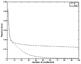
In Figures
8
and
9 we
show how the 95th percentile of the relative error across all the ports
decreases as a function of the number of coefficients used for
representing the traffic data for each port for TCP and UDP ports
respectively. We find that after 30-35 coefficients we gain little by
adding additional coefficients, i.e., the marginal improvement in the
fidelity of the representation becomes less significant. We will
address this issue again in Section
8, by
considering the rate of decrease of the residual as a function of the
number of modes selected for specific ports, to derive stopping criteria
for obtaining compressed representations.
Figure 8: 95th percentile of
relative error vs. number of coefficients selected for TCP ports
(incoming flows)
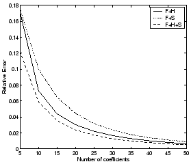 |
Figure 9: 95th percentile of
relative error vs. number of coefficients selected for UDP ports
(incoming flows)
 |
6.3 Analysis of Selected Modes
We proceed to analyze the set of dictionary components that are chosen
in the compressed representation using the redundant dictionaries for
different ports, along different spatial and temporal dimensions.
First, we are interested to see if there is substantial similarity in
the set of dictionary components selected in the compressed
representation across different ports. Second, we want to observe the
temporal properties of compression; i.e., for a fixed traffic dimension,
how does one week differ from another in terms of the components
selected from the redundant dictionary? Third, we want to identify
possible sources of correlation across the different traffic aggregates
(flows, packets, bytes, both to and from) on a particular port of
interest. Such analysis not only helps us to understand the nature of
the underlying constituent components that make up each traffic time
series but also enables us to identify possible sources of joint
compression, to further reduce the storage requirements. For the
discussion presented in this section, we use the dictionary
(Fourier + Spike) as the redundant dictionary for our
analysis.
We observe that the majority of selected dictionary components are
restricted to a small number of ports--this is expected as these modes
capture the minor variations across different ports, and also represent
traffic spikes that may be isolated incidents specific to each port. We
also observe that there are a few components that are consistently
selected across almost all the ports. These components that are present
across all the ports under consideration include the mean (zero-th
Fourier component), the diurnal/off-diurnal periodic components, and a
few other periodic components which were found to be the highest energy
components in the Fourier analysis presented in Section
6.1.
6.3.2 Temporal Analysis Across Multiple Weeks
We also analyze, for specific instances of ports as defined by our four
categories, the temporal stability of the set of components that are
selected across different weeks over the 20 week data set, using 30
modes per week. As before, we use
as the
redundant dictionary for compression. For each dictionary component
(periodic component or spike) that is selected in the compressed
representation over the 20 week period, we count the number of weeks in
which it is selected. We show in Figure
10 the number
of components that have an occurrence count more than

, as
a function of
. We observe that the majority of the
components are selected only for 1-2 weeks, which indicates that these
captured subtle traffic variations from week to week. To further
understand the stability of the components, we divide them into 3
categories: components that occur every week, components that occurred
greater than 50% of the time (i.e, were selected 10-20 times over the 20
week period), and components that occurred fewer than 50% of the time
(i.e., fewer than 10 times). Table
2 presents the
breakdown for the above classification for different ports in each
category, and also shows the type of components that occur within each
count-class. We find that across all the ports, the dictionary
components that are always selected in the compressed representation
correspond to periodic components such as the diurnal and off-diurnal
frequencies.
Figure 10: Occurrence counts
using a 30 coefficient representation with :Fourier+Spike
over a 20 week period
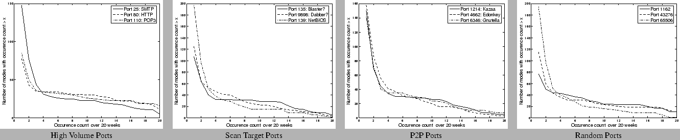 |
Table 2: Analyzing stable dictionary
components for different classes of ports
| Port
Type |
Port
Number |
All 20 weeks |
10-20 weeks |
0-10 weeks |
| Periodic |
Spike |
Periodic |
Spike |
Periodic |
Spike |
| High
Volume |
25 |
5 |
0 |
18 |
0 |
23 |
102 |
| 80 |
11 |
0 |
19 |
0 |
15 |
33
|
| P2P |
1214 |
5 |
0 |
21 |
0 |
20 |
104 |
| 6346 |
7 |
0 |
17 |
0 |
23 |
94
|
| Scan |
135 |
5 |
0 |
24 |
0 |
15 |
63 |
| 9898 |
3 |
0 |
20 |
0 |
35 |
67
|
| Random |
5190 |
11 |
0 |
10 |
0 |
27 |
73 |
| 65506 |
1 |
0 |
15 |
0 |
31 |
147
|
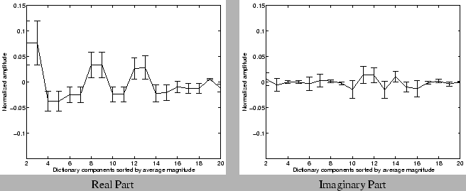
The stability of a component depends not only on the fact that it was
selected in the compressed representation, but also on the amplitude of
the component in the compressed representation. Hence, we also analyze
the amplitudes of the frequently occurring components (that occur
greater than 50% of the time) across the 20 week dataset. Figures
11 and
12 show the mean
and deviation of the amplitudes returned by the greedy pursuit
procedure for these frequently occurring components. For clarity, we
show the amplitudes of the real and imaginary part of the Fourier
(periodic) components separately. For each port, we first sort the
components according to the average magnitude (i.e, the energy
represented by both the real and imaginary parts put together) over the
20 week period. We normalize the values of the average amplitude in both
real and imaginary parts, and the deviations by the magnitude of the
mean (or zero-th Fourier) component. We observe that the amplitudes are
fairly stable for many Fourier components across the different port
types. These results suggest that these stable (Fourier) frequencies may
indeed form fundamental components of the particular traffic time
series. The relative stability of amplitudes in the compressed
representation also indicates that it may be feasible to build traffic
models, that capture the fundamental variations in traffic, using the
compressed representations.
Figure 11: Stability of
amplitudes of dictionary components selected - High volume: Port 80
 |
Figure 12: Stability of
amplitudes of dictionary components selected - P2P Port: 1214
 |
6.3.3 Spatial Analysis Across Traffic Metrics
The last component of our analysis explores the similarity in the
traffic data across different aggregates for a given port, within each
week. One naturally expects a strong correlation between the number of
flows, the number of packets, and the number of bytes for the same port,
and also reasonable correlation between the total incoming volume and
the total outgoing volume of traffic on the same port
4.
Figure
13
confirms this natural intuition about the nature of the traffic
aggregates. We observe that for the high volume and P2P application
ports, more than two-thirds of the dictionary components are commonly
selected across all the different traffic aggregates and we also find
that more than 30 components are selected across at least 4 of the
traffic aggregates (bytes, packets, flows both to and from the port). We
found that such similarity in the selected components across the
different aggregates is less pronounced for the scan target ports and
the random ports under consideration. Our hypothesis is that the
distribution of packets per flow and bytes per packet are far more
regular for the high volume applications (for example most HTTP, P2P
packets use the maximum packet size to get maximum throughput) than on
the lesser known ports (which may be primarily used as source ports in
small sized requests).
Figure 13: Occurrence counts
using 30 coefficient representation with :Fourier+Spike
over different traffic aggregates for a single week
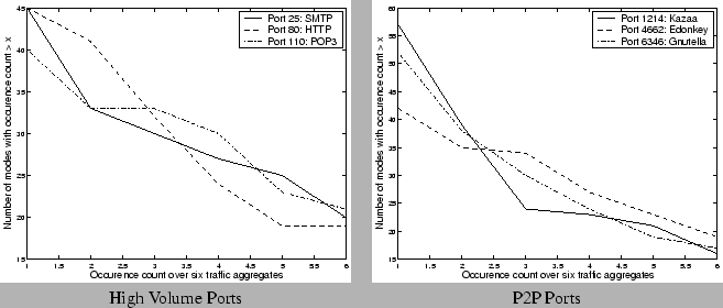 |
7 Applications
7.1 Visualization
One of the primary objectives of compression is to present to the
network operator a high fidelity approximation that captures salient
features of the original traffic metric of interest. Visualizing
historical traffic patterns is a crucial aspect of traffic monitoring
that expedites anomaly detection and anomaly diagnosis involving a
network operator, who can use historical data as visual aids. It is
therefore imperative to capture not only the periodic trends in the
traffic, but also the isolated incidents of interest (for example, a
post-lunch peak in Port 80 traffic, the odd spike in file sharing
applications, etc).
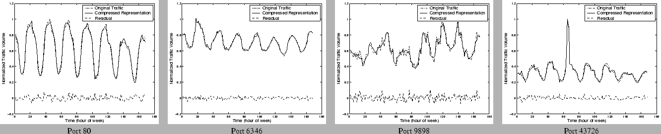
Figure 14 shows
some canonical examples from each of the four categories of ports we
described earlier. In each case we show the original traffic time series
over a week and the time series reconstructed from the compressed
representation using 1:6 compression with (Fourier +
Haar + Spike). We also show the residual signal, which is the point-wise
difference between the original signal and the compressed
reconstruction. The traffic values are normalized with respect to the
maximum traffic on that port observed for the week. We find that the
compressed representations provide a high fidelity visualization of the
original traffic data. Not surprisingly, the ports which exhibit the
greatest amount of regularity in the traffic appear to be most easily
compressible and the difference between the actual and compressed
representation is almost negligible for these cases. It is also
interesting to observe in each case that the compressed representation
captures not only the periodic component of the signal, but also traffic
spikes and other traffic variations.
Figure 14: Miscellaneous
Ports using : Fourier + Haar Wavelets + Spikes
 |
7.2 Traffic Trend Analysis
Analyzing trends in traffic is a routine aspect in network operations.
Operators would like to understand changes and trends in the application
mix that is flowing through the network (e.g. detecting a a new popular
file sharing protocol). Understanding traffic trends is also crucial for
traffic engineering, provisioning, and accounting applications. It is
therefore desirable that such trend analysis performed on the compressed
data yields accurate results when compared to similar trend analysis on
the raw (uncompressed) data. A simple method to extract trends over
long timescales is to take the weekly average, and find a linear fit
(using simple linear regression to find the slope of the line of best
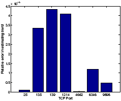
fit) to the weekly averages over multiple weeks of data. In Figure
15, we plot the
relative error in estimating such a linear trend. We estimate the trend
using 20 weeks of data for different ports, and in each case we
estimate the slope of the best linear fit on the raw data and on the
compressed data (using a 30 coefficient representation using
). We observe that across the different ports, the
relative error in estimating the trend is less than 0.5%, which
reaffirms the high fidelity of the compression techniques.
Figure 15: Relative error in
estimating traffic trends
 |
We observed in Section
6.3 that the
underlying fundamental components are stable (both in terms of
occurrence and their amplitudes) over time. It is conceivable that
traffic models for anomaly detection can be learned on the compressed
data alone. Our initial results suggest that traffic models [
15] learned from
compressed data have almost identical performance to models learned from
uncompressed data, and hence compression does not affect the fidelity of
traffic modeling techniques. Ongoing work includes evaluating different
models for building prediction models for real-time anomaly detection
using accurate yet parsimonious prediction models generated from the
insights gained from the compression procedures.
8 Discussion
In our experiments, we fixed the number of coefficients across all
ports. One can imagine a host of stopping criteria to apply. One
particularly interesting observation is that in many of the cases, a few
of which are depicted in Figure
16, we find
that the residual energy has a distinct knee beyond which the rate of
drop in the residual energy is significantly lower. Intuitively one can
imagine as the knee corresponding to the stochastic noise component of
the original signal, which cannot be efficiently represented using any
fundamental component. Note that the anomalous incidents such as spikes
or glitches are usually captured before we hit the knee of the curve, as
observed in Section
7.1. This raises
the possibility that we have a
robust representation of the
original signal--one that does not change with the addition of noise as
there are diminishing returns for any added effort aimed at modeling the
noise component, which are not necessarily of interest either from a
visualization or modeling perspective.
Figure 16: Evaluating
Stopping Criteria: Relative Error vs. number of coefficients
 |
We have performed independent experiments with synthetic time series
signals, similar to traffic time series (sinusoidal signals, with spikes
and different noise patterns thrown in). We observe that in almost all
the cases we observe a distinct knee in the redundant dictionary
decomposition, once the fundamental high energy components get picked.
We also find that the asymptotic slope of the curve of the residual
energy beyond the knee has a unique signature that is characterized by
the nature of the noise component (Gaussian or ``White'' vs. Power-law
or ``Colored''), and the redundant dictionary used.
8.2 Smaller Scales
At an appropriate aggregation level, network traffic will exhibit some
periodicities. Traffic time series data from a variety of settings
(enterprise and university) also confirm this hypothesis. These data
typically represent the aggregate traffic at the border of a reasonably
large network with fairly high aggregation levels. We believe that the
methods for time-series compression using matching pursuit with
redundant dictionaries are still applicable to data even at slightly
lower scales of aggregation.
One of the objectives of compressing the time series is to enable
different scales of time resolution for anomaly detection. It is
imperative that the time scale for detecting traffic anomalies be less
than the minimum time required for a large network attack to saturate.
When the compression is applied to traffic aggregates at finer time
granularities (e.g. for each week if we had volume counts for each five
minute bin instead of hourly time bins), one expects that the effective
compression would be better. The rationale behind the intuition arises
from the fact that the high energy fundamental components correspond to
relatively low frequency components, and such pronounced periodicities
are unlikely to occur at finer time-scales. As a preliminary
confirmation of this intuition, we performed the same compression
procedures on a different data set, consisting of 5 minute traffic rates
collected from SNMP data from a single link. Note that with 5-minute
time intervals, we have 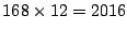 data points per week. Figure 17 the relative error as
a function of the number of coefficients used in the compressed
representation (using ). We observe that with
less than 40 ( = 2% of the original space requirement) coefficients we
are able to adequately compress the original time-series (with a
relative error of less than 0.005), which represents significantly
greater possible compression than those observed with the hourly
aggregates.
data points per week. Figure 17 the relative error as
a function of the number of coefficients used in the compressed
representation (using ). We observe that with
less than 40 ( = 2% of the original space requirement) coefficients we
are able to adequately compress the original time-series (with a
relative error of less than 0.005), which represents significantly
greater possible compression than those observed with the hourly
aggregates.
Figure 17: Compressing SNMP
data collected at five minute intervals from a single link
 |
8.3 Encoding Techniques
We observed that with larger dictionaries that include full-translation
wavelets, we can achieve better compression. There is, however, a
hidden cost in the effective compression with larger dictionaries as the
indices of a larger dictionary potentially require more bits to
represent than the indices of a smaller dictionary. One can imagine
better ways of encoding the dictionary indices (e.g., using Huffman
coding) to reduce the amount of space used up for storing the dictionary
indices in addition to the component amplitudes. Our work explored the
potential benefit of using signal processing methods for lossy
compression and we observed that there is a substantial reduction in the
storage requirement using just the methods presented in this paper. Many
compression algorithms use lossy compression techniques along with
efficient encoding techniques (lossless compression) to get the maximum
compression gain, and such combinations of lossy and lossless
compression methods can be explored further.
8.4 Joint Compression
We observe that there are multiple sources of correlation across the
different traffic dimensions that may be additionally utilized to
achieve better compression. The temporal stability of the compressed
representations (Section
6.3.2) suggests
there is scope for exploiting the similarity across different weeks for
the same traffic aggregate. For example, we could build a stable model
over
weeks of data for each port/prefix and only
apply the sparse approximation to the difference of each particular week
from the model. Alternately one could imagine applying the simultaneous
compression algorithms [
16] across the
different weeks for the same port. The simultaneous compression
algorithms approximate all these signals at once using different linear
combinations of the same elementary signals, while balancing the error
in approximating the data against the total number of elementary signals
that are used. We also observed that there is reasonable correlation in
spatial dimensions, since the compressed representation of different
traffic aggregates such as flows, packets, and bytes show significant
similarity (Section
6.3.3).
The observations of the low dimensionality of network traffic data
across different links also raises the possibility of using Principal
Component Analysis (PCA) [10] for
extracting better spatial compression, both across different traffic
aggregates (e.g. different ports, across time) and across different
measurements (e.g. across per-link, per-router counts). PCA like methods
can be used to extract the sources of correlation before one applies
redundant dictionary approaches to compress the traffic data. For
example we can collapse the 20 week data set for a single port into a
single matrix of traffic data, on which PCA like techniques can be
applied to extract the first few common components, and the redundant
dictionary can be applied on the residual (the projection on the
non-principal subspace) to obtain a higher fidelity representation.
9 Conclusions
There is a pressing need for fine-grained traffic analysis at different
scales and resolutions across space and time for network monitoring
applications. Enabling such analysis requires the ability to store large
volumes of historical data across different links, routers, and
customers, for generating visual and diagnostic aids for network
operators. In this paper, we presented a greedy pursuit approach over
redundant dictionaries for compressing traffic time series data, and
evaluated them using measurements from a large ISP. Our observations
indicate that the compression models present a high fidelity
representation for a wide variety of traffic monitoring applications,
using less than 20% of the original space requirement. We also observe
that most traffic signals can be compressed and characterized in terms
of a few stable frequency components. Our results augur well for the
visualization and modeling requirements for large scale traffic
monitoring. Ongoing work includes evaluating and extracting sources of
compression across other spatial and temporal dimensions, and evaluating
the goodness of traffic models generated from compressed
representations.
-
- 1
- BARFORD, P., KLINE, J., PLONKA,D.,AND
RON,A.
A Signal Analysis of Network Traffic Anomalies.
In Proc. of ACM/USENIX Internet Measurement Workshop (2002).
- 2
- DUFFIELD, N. G., LUND, C., AND
THORUP,M.
Charging From Sampled Network Usage.
In Proc. of ACM SIGCOMM Internet Measurement Workshop (2001).
- 3
- ESTAN, C., SAVAGE, S., ANDVARGHESE,G.
Automatically Inferring Patterns of Resource Consumption in Network
Traffic.
In Proc. of ACM SIGCOMM (2003).
- 4
- FROSSARD, P., VANDERGHEYNST, P., I VENTURA,R.
M. F., AND KUNT, M.
A posteriori quantization of progressive matching pursuit streams.
IEEE Trans. Signal Processing (2004), 525-535.
- 5
- GILBERT, A. C., MUTHUKRISHNAN, S.,AND
STRAUSS,M. J.
Approximation of functions over redundant dictionaries using coherence.
In Proc. of 14th Annual ACM-SIAM Symposium on Discrete Algorithms
(2003).
- 6
- GRIBONVAL, R., AND BACRY, E.
Harmonic decomposition of audio signals with matching pursuit.
IEEE Trans. Signal Processing (2003), 101-111.
- 7
- INDYK, P.
High-dimensional computational geometry.
PhD thesis, Stanford University, 2000.
- 8
- KRISHNAMURTHY, B., SEN, S., ZHANG,Y.,AND
CHEN,Y.
Sketch-based Change Detection: Methods, Evaluation, and Applications.
In Proc. of ACM/USEINX Internet Measurement Conference (2003).
- 9
- LAKHINA, A., CROVELLA, M., AND
DIOT,C.
Diagnosing network-wide traffic anomalies.
In Proc. of ACM SIGCOMM (2004).
- 10
- LAKHINA, A., PAPAGIANNAKI, K., CROVELLA,M.,
DIOT, C., KOLACZYK, E., AND TAFT,N.
Structural analysis of network traffic flows.
In Proc. of ACM SIGMETRICS (2004).
- 11
- LEMPEL, A., AND ZIV, J.
Compression of individual sequences via variable-rate coding.
IEEE Transactions on Information Theory 24, 5 (1978),
530-536.
- 12
- MALLAT, S., AND ZHANG, Z.
Matching pursuits with time frequency dictionaries.
IEEE Trans. Signal Processing 41, 12 (1993), 3397-3415.
- 13
- MILLER, A. J.
Subset selection in regression, 2nd ed.
Chapman and Hall, London, 2002.
- 14
- Cisco Netflow.
https://www.cisco.com/warp/public/732/Tech/nmp/netflow/index.shtml.
- 15
- ROUGHAN, M., GREENBERG, A., KALMANEK,C.,
RUMSEWICZ, M., YATES, J., AND ZHANG,Y.
Experience in measuring internet backbone traffic variability: Models,
metrics, measurements and meaning.
In Proc. of International Teletraffic Congress (ITC) (2003).
- 16
- TROPP, J. A., GILBERT, A. C.,ANDSTRAUSS,M. J.
Algorithms for simultaneous sparse approximation part i: Greedy
pursuit.
submitted (2004).
- 17
- ZHUANG, Y., AND BARAS, J. S.
Optimal wavelet basis selection for signal representation.
Tech. Rep. CSHCN TR 1994-7, Institute for Systems Research, Univ. of
Maryland, 1994.
Notes
- Typically, k is less than k, i.e. the magnitudes of the
amplitudes of the dictionary components are less than the original time
series.
- The slowest step in OMP is choosing the waveform which
maximizes the dot product with the residual at each step. We can speed
up this step with a Nearest Neighbors data structure [7] and reduce the
time complexity for each iteration to N + polylog(d).
- Note that for each Fourier coefficient, we need to store both the
real part and the imaginary part. It appears that we may actually need
twice the space. However, the amplitudes for frequency f and frequency
-f are the same (except that they are complex conjugates of one
another), we can treat them as contributing only two coefficients to the
compressed representation together in total as opposed to four
coefficients.
- We however note that there may be certain exceptional situations
(e.g., worm or DDoS attacks that use substantially different packet and
byte types) where such stable correlations between the flow,
packet, and byte counts may not always hold.
Footnotes
- ... Aiello
- Majority of this work was done when the author was a member of
AT & T Labs-Research
- ... Gilbert
- Majority of this work was done when the author was a member of
AT & T Labs-Research. The author is supported by an
Elizabeth Crosby Faculty Fellowship.
- ... Sekar
- Majority of this work was done when the author was a research
intern at AT & T Labs-Research