IMC '05 Paper
[IMC '05 Technical Program]


An Information-theoretic Approach to Network Monitoring and Measurement
Yong Liu
ECE Dept.
Polytechnic University
Brooklyn, NY 11201
-
Don Towsley
Dept. of Computer Science
University of Massachussetts
Amherst,
MA 01003
-
Tao Ye
Sprint ATL
Burlingame, CA 94010
-
Jean Bolot
Sprint ATL
Burlingame, CA 94010
Network engineers and operators are faced with a number of
challenges that arise in the context of network monitoring and
measurement. These include: i) how much information is included
in measurement traces and by how much can we compress those
traces?, ii) how much information is captured by different
monitoring paradigms and tools ranging from full packet header
captures to flow-level captures (such as with NetFlow) to packet
and byte counts (such as with SNMP)? and iii) how much joint
information is included in traces collected at different points
and can we take advantage of this joint information? In this
paper we develop a network model and an information theoretic
framework within which to address these questions. We use the
model and the framework to first determine the benefits of
compressing traces captured at a single monitoring point, and we
outline approaches to achieve those benefits. We next consider
the benefits of joint coding, or equivalently of joint compression
of traces captured a different monitoring points. Finally, we
examine the difference in information content when measurements
are made at either the flow level or the packet/byte count level.
In all of these cases, the effect of temporal and spatial
correlation on the answers to the above questions is examined.
Both our model and its predictions are validated against
measurements taken from a large operational network.
Network monitoring is an immense undertaking in a large network.
It consists of monitoring (or sensing) a network using a
geographically distributed set of monitoring stations, with the
purpose of using the monitoring data to better understand the
behavior of the network and its users. Monitoring is a central
activity in the design, engineering, and operation of a network.
Increased monitoring capabilities, along with the associated
increased understanding of the network and user behavior (or
misbehavior), have direct impact on network performance and
integrity, and therefore on the costs passed on to network users,
and on the revenues of the operators. In spite of its
importance, practitioners struggle with challenging,
yet very practical questions such as
where within the network to monitor data and at what granularity
to capture traces, how much information is included in various types of packet
traces and by how much can we compress those
traces, and how much joint information is included in
traces collected at different points and how can we
take advantage of this joint information?
In this paper, we address these questions in the context of
large high speed networks such as campus, enterprise, or core
networks. Monitoring the behavior of such networks raises tremendous
challenges due to the high bandwidth of currently deployed links.
For example, the collection of 60-byte packet headers can easily
generate 3Tb of data per hour on a OC-192 link (10 Gb/s link) in a
core backbone, and 30Gb of data per hour at an enterprise or campus
gateway. One means for reducing the amount of data gathered is to
monitor flow-level data, as is done with Net Flow [2].
The amount of data can be further
reduced by monitoring packet or byte counts over fixed intervals of
time as is possible using SNMP [15]. Network data collected at
distributed monitors also exhibit spatial and temporal correlations.
Thus another means for reducing the sizes of monitored data sets is
to exploit this correlation through correlated data coding and compression.
In this paper, we propose an information theoretic framework
within which to address some of the issues and questions introduced
above. In particular, we propose and validate a flow-level model
(adapted from [12]), and we use it to determine the information
content of a packet trace collected at a single or multiple points in a network, and
of sets of packet traces collected at separate points. We also
determine the information content of traces captured at different
levels of granularity, in particular flow level traces (NetFlow
traces) and byte or packet count traces (SNMP traces).
We obtain a number of interesting and important results.
Regarding traces collected at a single monitoring point, we derive
an information theoretic bound for the information content in
those traces, or equivalently for the potential benefit of lossless
compression on those traces.
Not surprisingly, we find that the information content is small
in SNMP traces, higher in NetFLow traces, and extremely high
in full packet level traces.
More interestingly, we show that full packet header traces can be compressed in practice
down to a minimum of 20% of their original size, and that the amount of
compression is a function of the average flow size
traversing that node: the larger the average flow size, the
smaller the compression ratio.
Regarding traces collected at multiple monitoring points, we find
that joint coding or compression of traces further reduces
the marginally compressed traces at the individual monitors. Specifically,
the joint compression ratio (or equivalently,
the additional compression benefit brought by joint coding of
traces) is low for SNMP or byte/packet count traces, higher for NetFlow
or flow-level traces, and higher still for packet-level traces.
This means, for example, that joint coding is not really
useful for SNMP data collected from different monitoring
points and sent back to a NOC or central analysis station. Since
SNMP data reporting takes little bandwidth anyway, it
makes sense not to invest in sophisticated coding
techniques in this case. However, NetFlow or packet
header capture and reporting can require a significant
amount of bandwidth and storage. Our results show that,
in this case, joint coding techniques have the potential to significantly
reduce those bandwidth and storage requirements.
Information-theoretic concepts and approaches have been used in the past to
examine a wide variety of networking issues such as connectivity
[18] and traffic matrix estimation [26],
anomaly detection [16], and compact
traffic descriptors [8,24] for network dimensioning and
QoS monitoring.
However, to our knowledge, our attempt is the first to introduce a
framework within which to address all the questions of interest
here, namely trace coding, correlated and joint coding, and
trace content at multiple time scales.
There has been work on trace compression, however it has been
heuristic in nature. For example, work described in [14,23]
proposed heuristics based on storing and compressing packet
headers collected at a single monitor along with timing
information in the form of flow records. Trajectory sampling
exhibits some elements in common with distributed compression of
monitored data [7]. Also related is work in the area of
inverting sampled data, e.g., [9,11]. Indeed, sampling can be
thought of as a form of lossy compression and these papers are
concerned with decoding the resulting traces. There is also an
extensive body of work produced within the sensor networking and
distributed signal processing communities;
see [4,6] and their references for examples. However, much
of it is in the context of abstract models of how data is
produced, e.g., Gaussian random fields, and is not directly
applicable in the domain of network monitoring.
The rest of the paper is structured in three parts. In Section
2 we present the various elements of
our framework, including relevant concepts from information theory,
our network flow-level model, and the network traces that will be
used throughout the paper. In Section 3,
we describe the first application of our framework, specifically
we derive the information content of packet header traces
collected at a single monitoring station and examine the
benefits of trace compression in this case.
In Section 4, we examine the more general
problem of correlated, or joint, coding of trace
captured at several monitoring stations. Section
5 then applies the model
to determine the loss in information content when either flow-level (Net Flow)
or byte count (SNMP) summary is applied to the full trace.
Section 6 concludes the paper.
2 Methodologies
In this section we provide the foundation for the rest of the paper.
We begin by reviewing several concepts needed from information theory
(Section 2.1) that form the basis for exploring information
content in network traces. This is followed with a description of the
network flow model to which they will be applied (Section
2.2). The section ends with a review of
a collection of network traces used to validate and parameterize the
model (Section 2.3).
2.1 Some concepts from Information Theory
We begin by introducing the concepts of
entropy and entropy rate and their relation to data compression
[5].
Definition 1
Shannon entropy. Let  be a discrete random variable
that takes values from  . Let
 ,  .
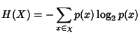
The entropy of is defined by
Examples of in our context would be the flow size measured
in packets, the flow identifier, and the packet/byte count in a one second interval.
Now consider a stochastic process
 where where
 is discrete valued. is discrete valued.
Definition 2
Entropy Rate.
The entropy rate of a discrete valued stochastic process is
defined by
when the limit exists.
The entropy rate represents the information rate conveyed by the
stochastic process . It provides an achievable lower bound on the
number of bits per sample required for lossless compression of the
process. With lossless compression, all of the information is
completely restored when the file is uncompressed. In our context,
an example might be the byte counts at a link over successive one
second intervals.
Definition 3
Joint Entropy Rate. The joint entropy rate of a
collection of many stochastic processes
 is defined by
 |
(1) |
when the limit exists.
The joint entropy rate represents the information rate conveyed
by the joint stochastic process and is an achievable lower bound
on the number of bits required per sample for the joint lossless
compression of all the processes.
Let us place this in our context. Let  be the header of the
  -th packet and -th packet and  the size of the
header. the size of the
header.
 is a stochastic process
representing packet headers. We are interested in quantifying the
benefit gained from compressing a packet header trace gathered
from one network monitor or traces collected at a set of network
monitors. is a stochastic process
representing packet headers. We are interested in quantifying the
benefit gained from compressing a packet header trace gathered
from one network monitor or traces collected at a set of network
monitors.
Definition 4
Marginal Compression Ratio. Given stationary stochastic
process
, the marginal compression ratio is
defined as the ratio of the entropy rate and record size,
In the case of traces collected at multiple points within the
network, we define:
Definition 5
Joint Compression Ratio. Given a collection of  jointly stationary stochastic
processes
 , the
joint compression ratio is defined as the ratio of the joint
entropy rate and the sum of the entropy rates of the individual
processes.
In the context of network trace compression, the joint compression
ratio quantifies the potential benefits of jointly compressing the
traces collected at several point in the network beyond simply
compressing each trace independent of each other.
Although much of the time we will deal with discrete random variables,
some quantities, such as interarrival times, are best approximated by
continuous random variables. This necessitates the following
definition.
Definition 6
Differential Entropy. Let be a continuous random
variable with a density  . The differential entropy of is
defined by
where  is the support set of the random variable.
In reality, every variable is measured with finite resolution.
With a resolution of
 , i.e., an , i.e., an  -bit
quantization, a continuous random variable is represented by a
discrete random variable -bit
quantization, a continuous random variable is represented by a
discrete random variable
 and its entropy is approximately and its entropy is approximately  . .
If follows an exponential distribution with rate  , its
differential entropy , its
differential entropy
With an n-bit quantization, the discrete entropy of is
 . In the following,
whenever there is no confusion, we use the notation . In the following,
whenever there is no confusion, we use the notation  for a
continuous random variable to represent its discrete entropy for a
continuous random variable to represent its discrete entropy
 . .
2.2 Network Flow Model
In this section we introduce a flow-based network model. We
represent the network as a directed graph  . Assume that
flows arrive to the network according to a Poisson process with
rate . Assume that
flows arrive to the network according to a Poisson process with
rate  and and  denotes the inter-arrival time
between flow denotes the inter-arrival time
between flow  and and  . Let . Let
 be the id
of the -th flow that arrives to the network. We assume that the
route of a flow be the id
of the -th flow that arrives to the network. We assume that the
route of a flow
 is fixed and classify flows into
non-overlap flow classes, is fixed and classify flows into
non-overlap flow classes,
 , such
that all flows within a class share the same route in the
monitored network. The route taken by flows in class is
represented by an ordered set , such
that all flows within a class share the same route in the
monitored network. The route taken by flows in class is
represented by an ordered set
 , where , where
 is the -th router traversed by a class flow
and is the -th router traversed by a class flow
and
 is the path length. The flow arrival
rate within class is is the path length. The flow arrival
rate within class is
 . When flow arrives, it
generates . When flow arrives, it
generates  packets. Packets within flow arrive according
to some point process with inter-arrival times packets. Packets within flow arrive according
to some point process with inter-arrival times
 , where , where
 is the
inter-arrival time between the is the
inter-arrival time between the  th and th packet of flow
. It is assumed that the first packet arrives at the same time
as the flow. The behavior of packet arrivals in the network is
described by the stochastic process th and th packet of flow
. It is assumed that the first packet arrives at the same time
as the flow. The behavior of packet arrivals in the network is
described by the stochastic process
 . .
Figure 1:
Experiment setup.
|
In practice, network traces are collected at distributed network
monitors. We are interested in how information is carried around
by packets when they traverse distributed network monitors. As a
starting point, we assume that there is no packet loss in the
network and packets incur constant delay on each link: let
 denote the delay that the denote the delay that the  -th packet incurs while
traversing the -th link, -th packet incurs while
traversing the -th link,
 , we assume that , we assume that
 , ,  . Delays are very small and losses non-existent
in a well-provisioned network such as the Sprint network.
Hence this is a reasonable assumption in many cases. In Section
4.3 we describe how these assumptions can be
relaxed. For a node . Delays are very small and losses non-existent
in a well-provisioned network such as the Sprint network.
Hence this is a reasonable assumption in many cases. In Section
4.3 we describe how these assumptions can be
relaxed. For a node  in the network, let in the network, let
 denote the set of flows that pass through it. Since flows arrive
to the network according to a Poisson process and the delay
between any two nodes in the network is constant, flows arrive to
node according to a Poisson process with rate
denote the set of flows that pass through it. Since flows arrive
to the network according to a Poisson process and the delay
between any two nodes in the network is constant, flows arrive to
node according to a Poisson process with rate
 . The behavior
of packet arrivals at node can be described by the stochastic
process . The behavior
of packet arrivals at node can be described by the stochastic
process
 , where , where
 is the sequence of inter-flow-arrival times
at node that follows exponential distribution with rate is the sequence of inter-flow-arrival times
at node that follows exponential distribution with rate
 , ,
 is an i.i.d. sequence of
flow ids seen by , is an i.i.d. sequence of
flow ids seen by ,
 is an i.i.d, sequence of
integer valued random variables that denote the number of packets
in the th flow passing through and is an i.i.d, sequence of
integer valued random variables that denote the number of packets
in the th flow passing through and
 is the sequence of flow
inter packet arrival times. is the sequence of flow
inter packet arrival times.
Figure 1 illustrates a simple scenario
corresponding to a router with two incoming links and two outgoing
links, each of which contains a monitor. There are four two hop paths
and four flow classes traversing these paths. This is the setting
within which the traces used for validation and parameterization of
the model are collected. They are described in the next section.
Figure 2:
Flow arrival is Poisson
|
2.3 Validation
The data used here were collected as part of the full
router experiment [13] on August 13, 2003. Packet traces
were recorded at six interfaces, i.e. 12 links of one gateway router
of the Sprint IP backbone network for 13 hours. We use mutually
synchronized DAG cards [1] to record packet headers with
GPS-precisioned 64bit timestamps from OC-3, OC-12 and OC-48 links
[10]. The experiment setup is shown in Figure 1.
In the remainder of this paper, we will focus on
the traces collected over a one hour time period between 14:30 and 15:30 GMT on
two incoming and two outgoing links. Table 1
summarizes the size of these traces and the link utilizations.
We choose this set of traces because it captures a mix of customer
to gateway and gateway to backbone traffic. Customer traffic
largely goes to one of the two backbone links. It is an ideal
first step to analyze information redundancy without being
overwhelmed by complicated routing. Furthermore, it is a
representative set of traffic data, because there are over 500
similarly configured gateway routers in Sprint's global network.
The shortcoming is that we do not have any backbone to backbone traffic
recorded at the same time. This will be considered in the
future work.
We further select the three most highly utilized links from the set to
use in the remainder of the paper. BB1-out, BB2-out are from two OC-48
linecards connecting to two backbone routers (BB1 and BB2). C1-in and C2-in
are from two OC-3 linecards connecting to transpacific customers.
We use the full packet trace to deduce an SNMP-like utilization
trace (refered to as utilization trace from now on) and an
unsampled raw Netflow trace. This is done so that different network
measurement techniques can be compared for the same time duration
without any possible measurement errors contributed by SNMP or
Netflow. The utilization trace is computed as byte-count per
second rather than per 5 minutes as a normal SNMP trace. This is
done to increase the number of data points and minimize estimation
error in the calculation. We simulate Netflow by creating an
unsampled Netflow trace from the packet trace, because we prefer
to not take into account packet sampling's effect on measurement
at this stage.
Table 1:
Trace description and stats.
| Data Set |
duration |
#packets |
Average rate |
| C1-in |
1 hour |
44,598,254 |
53Mbps |
| C2-in |
1 hour |
123,542,790 |
73Mbps |
| BB1-out |
1 hour |
71,115,632 |
69Mbps |
| BB2-out |
1 hour |
105,868,070 |
82Mbps |
|
The full packet traces described above are used to validate the
Poisson assumptions made in the flow model. Figure
2 depicts a QQ plot of the empirical inter-flow
arrival time distribution with respect to an exponential distribution
with the same average. We observe visually a good match for the flow
inter-arrival times associated with link C1-in. This is also
the case with the other flow arrival traces and is consistent with
observations made elsewhere [12]. We compute empirical
entropy on the traces described above using empirical marginal
probability distributions.
3 Application: Single Point Trace Compression
All packet monitoring poses tremendous challenges to the storage
subsystems due to the high volume of current network links.
We use the information theoretic approach to identify and quantify the
potential benefit of network trace compression based on the network
flow model. In this section, we focus on full trace collection at a single monitor such as an IPMON system [10]. We start with
calculating the information content in traces made of packet headers.
It will become clear that the
temporal correlation resulted from the flow structure leads to
considerable marginal compression gain. We then show by empirical
study that other fields in IP header will contain no/very small amount
of information. We conclude this section with guidelines for the
development of practical network trace compression algorithms. The
next section concerns the simultaneous collection of traces at
multiple monitors distributed throughout a network.
Table 2:
Comparision of entropy calculations and real compression algorithm gain
| Trace |
 |
 |
 |
 |
 |
 |
 |
Compression |
| |
bin=8 s s |
bin=2pkts |
bin=128s |
|
|
|
|
Algorithm |
| C1-in |
8.8071 |
3.2168 |
9.7121 |
104 |
21.0039 |
706.3772 |
0.2002 |
0.6425 |
| BB1-out |
7.6124 |
2.4688 |
12.1095 |
104 |
20.4825 |
736.1722 |
0.2139 |
0.6574 |
| BB2-out |
7.1594 |
2.7064 |
12.4824 |
104 |
18.7890 |
689.9066 |
0.2186 |
0.6657 |
|
3.1 Entropy of Flow-based Trace
In the IPMON style full packet header trace capture system, The IP
header and additional TCP/UDP header of each packet is stored in the
trace. Here we only concern with the information content in
the IP header, and leave TCP/UDP header for future work (except the
port fields). We start with
calculating the information content in packet time-stamp and 5-tuple flow ID.
The total length of an uncompressed timestamp is
 . The behavior of packet arrivals in the network is described
by the stochastic process
(to avoid triviality, we assume . The behavior of packet arrivals in the network is described
by the stochastic process
(to avoid triviality, we assume
 ). We are interested in determining the minimum number
of bits required to represent each flow. If we assume flow
inter-arrival ). We are interested in determining the minimum number
of bits required to represent each flow. If we assume flow
inter-arrival
 , flow Id , flow Id
 and packet
inter-arrivals within a flow
are
pairwise independent, on average we need a number of bits per flow
equal to and packet
inter-arrivals within a flow
are
pairwise independent, on average we need a number of bits per flow
equal to  where where
 |
(2) |
where
 denotes the information content in
packet inter-arrivals within a flow. It can be shown that denotes the information content in
packet inter-arrivals within a flow. It can be shown that
where  represents the inter-arrival time
between randomly picked adjacent packet pairs from all flows.
Inequality (5) is an equality if packet
inter-arrival times within a flow, represents the inter-arrival time
between randomly picked adjacent packet pairs from all flows.
Inequality (5) is an equality if packet
inter-arrival times within a flow,
 , are i.i.d.
sequence. Inequality (6) is an equality if packet
inter-arrival times are independent of flow size , are i.i.d.
sequence. Inequality (6) is an equality if packet
inter-arrival times are independent of flow size  . .
Figure 3:
Flow size correlation with inter-packet arrival time within
a flow. Larger flow size correspond to shorter inter-packet arrival times.
[scale=0.35]figs/sj07_flowsize_pktia.eps
|
Fig. 3 shows there is in fact a strong
correlation between flow size and inter-packet arrivals time
within a flow. Large flows with many packets tend to have smaller
inter-packet arrival times. This suggests there is opportunity in
further compressing the inter-packet arrival time within a flow.
However the Inequality (6) provides us with an upper
bound in compression ratio.
The per-flow information consists of two parts: one part is timing
information about the flow arrival and flow ID, which is shared by
all packets in the flow; the other part consists of all the packet
inter-arrival information, which grows sub-linearly with the
number of packets within the flow if we assume packet
inter-arrivals are dependent. (Note: If packet inter-arrival
times are independent it grows linearly.) The information rate per
unit time is then
 . .
There exists other fields in the IP header as well, such as TOS,
datagram size, etc. A detailed study in [19] shows that they carry
little information content in the framework of the flow model, and can
be modeled similarly to the packet inter-arrival time within a flow.
We therefore take the simplified approach and only consider the
timestamp field and the flow ID field in this paper.
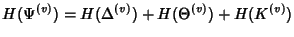
In practice, traces are
collected at individual nodes. For a node in the network, we
need a number of bits per flow equal to
 where where
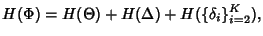
![\begin{displaymath}\begin{split}H(\Phi^{(v)}) & \leq H(\Theta^{(v)})+ H(\Delta^{(v)}) + H(K^{(v)})\\ & +(E[K^{(v)}]-1) H(\delta^{(v)}) \end{split}\end{displaymath}](img89.png) |
(7) |
As before the inequality
becomes equality when
 is independent of is independent of
 and the latter sequence is iid. and the latter sequence is iid.
The information rate per unit time is then
 at node . In the absence of compression, each
flow requires on average at node . In the absence of compression, each
flow requires on average
![$ (104 + 64)E[K^{(v)}]$](img93.png) bits with bits with  bits to encode the 5-tuple flow identifier and bits for
timestamps of packet arrivals.
bits to encode the 5-tuple flow identifier and bits for
timestamps of packet arrivals.
Now we can answer the question: what is the maximum benefit that
can be achieved through compression? From
 , we have a
marginal compression ratio , we have a
marginal compression ratio
![$\displaystyle \rho (\Phi^{(v)})= \frac{H(\Phi^{(v)})}{168*E[K^{(v)}]}\\ $](img96.png) |
(8) |
The compression ratio
 provides a lower bound on what can be achieved
through lossless compression of the original network trace. From
(7) and (8), the marginal
compression ratio at a node is a decreasing function of provides a lower bound on what can be achieved
through lossless compression of the original network trace. From
(7) and (8), the marginal
compression ratio at a node is a decreasing function of
![$ E[K^{(v)}]$](img98.png) , the average size of flows traversing that node.
Since the information in flow ID , the average size of flows traversing that node.
Since the information in flow ID
 and flow arrival and flow arrival
 is shared by all packets in the flow, the
larger the average flow size, the smaller the per-packet share,
therefore the smaller the compression ratio. When
is
large, the compression ratio is bounded from below by is shared by all packets in the flow, the
larger the average flow size, the smaller the per-packet share,
therefore the smaller the compression ratio. When
is
large, the compression ratio is bounded from below by
![$ (E[H(\delta^{(v)})])/168$](img101.png) , which is an indication of how
compressible the packet inter-arrival time is in average. (Note:
this bound results from the assumption that packet inter-arrival
times within a flow are independent. If there is correlation
between packet inter-arrival times, a tighter bound can be derived
to explore the correlation.) Therefore, the marginal
compression ratio for long flows is determined by the compression
ratio of packet inter-arrival times. , which is an indication of how
compressible the packet inter-arrival time is in average. (Note:
this bound results from the assumption that packet inter-arrival
times within a flow are independent. If there is correlation
between packet inter-arrival times, a tighter bound can be derived
to explore the correlation.) Therefore, the marginal
compression ratio for long flows is determined by the compression
ratio of packet inter-arrival times.
3.3 Results
We summarized the marginal compression ratio for a single trace in
Table 2. We compare the compression upperbound
from the flow model entropy calculation and a practical trace compression
algorithm. The trace compression software is an implementation of
the schemes introduced in [14]. The practical
algorithm uses a flow-based compressed scheme very similar to the flow
model in section 2.2. It does, however,
record additional IPID, datagram size and TCP/UDP fields in each
packet of a flow.
For the three traces we considered, the entropy calculation suggests a
bound of compression ratio 20.02% to 21.86% of the original
trace. However the practical scheme only compresses 64.25% to 66.57%
of the original trace. The most significant algorithm difference is
that this scheme keeps a fixed packet buffer for each flow, therefore
records very long flows as many smaller flows. This is done for the
ease of decompression and quickly count for very long flows, avoiding
only outputting long flows after they end. This could result in long
flows being broken down to many small flows and duplicate the flow
record many times, therefore reducing the compression benefits.
4 Application: Joint Trace Coding
The fact that one flow traverses multiple monitors introduces
spatial correlation among traces collected by distributed
monitors. We calculate the joint entropy of network traces which
serves as the lower bound for distributed traces compression. To
account for network uncertainties, such as packet loss and random
delay, we incorporate additional terms to characterize
network impairment.
We are interested in quantifying how well marginal compression
comes to achieving the entropy rate of the network. We have
where the numerator is the lower bound on joint compression and
the denominator is the lower bound of marginal compression of each
trace separately. The joint compression ratio  shows the
benefit of joint compression. shows the
benefit of joint compression.
The entropy of a flow record of class can be calculated as
 . The information rate generated by
flow class is . The information rate generated by
flow class is
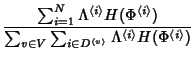
 . Therefore, the network information rate is: . Therefore, the network information rate is:
 |
(10) |
At node , denote by
 the set of flow classes traversing it. The total
information rate at is the set of flow classes traversing it. The total
information rate at is
 |
(11) |
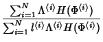
Plugging (10) and (11) into
(9), we have
It suggests that the joint compression ratio is
inversely proportional to a weighted average of the number of
monitors traversed by flows. Intuitively, all monitors traversed
by a flow collect redundant information for that flow. The longer
the flows paths, the higher the spatial correlation in distributed
packet header traces, the bigger the potential gain of distributed
trace compression.
Table 3:
Joint trace compression ratio
| |
Joint Compression Ratio |
 (C1-in, BB1-out, C2-in, BB2-out) (C1-in, BB1-out, C2-in, BB2-out) |
0.5 |
| (C1-in to BB1-out) |
0.8649 |
| (C1-in to BB2-out) |
0.8702 |
| (C2-in to BB1-out) |
0.7125 |
| (C2-in to BB2-out) |
0.6679 |
|
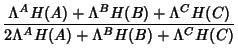
According to (9), the joint compression ratio for
all the links traversing through our router is simply 0.5, since
the path length ( ) is 2 for each flow class. We're also
interested in knowing the joint compression ratio of a path
connecting any two links. For example, let us denote the flow
classes C1-in to BB1-out as A, C1-in to BB2-out as B, and C2-in to
BB1-out as C, the compression ratio for the path through links
C1-in and BB1-out is: ) is 2 for each flow class. We're also
interested in knowing the joint compression ratio of a path
connecting any two links. For example, let us denote the flow
classes C1-in to BB1-out as A, C1-in to BB2-out as B, and C2-in to
BB1-out as C, the compression ratio for the path through links
C1-in and BB1-out is:
The results in Table 3 show a substantial 50% to
87% joint compression ratio over multiple monitoring points.
The ratio is lower (namely 0.5) when computed across all monitors from the same
router, and higher (namely 0.6679 to 0.8702) when computed over only
two links. The savings come from a significant amount of shared flows in these
monitoring points. This
suggests that if we can successfully share information at the
correlated monitoring points and perform joint coding, the potential
savings will be very significant. In practice, it could be difficult to
devise a perfect coding scheme for the entire network. We leave this
for a future direction.
4.3 Network Impairments
Till now we have assumed that link delays are constant and that
there are no packet losses. These can be accounted for by
augmenting the expression for the flow entropy to account for
these. Take the case where link delays are not constant as an
example. Due to variable link delays, the inter-arrival time of
two adjacant packets within a flow varies when they traverse the
network. Link delays may also induce packet reordering. To fully
capture the timing information of all packets in the network,
one will have to record not only the packet inter-arrival time within
a flow at their network entry point, but also the packet delays on all
links. Suppose for now that the delay sequences
 ,
are mutually
independent sequences of iid rvs. Then becomes
where ,
are mutually
independent sequences of iid rvs. Then becomes
where  is given by (2) and is given by (2) and  is
Note that in the case that link delays are correlated, this
provides an upper bound. Figure 4 plots the
distribution of the single hop packet delay on an operational
router in Sprint Network. The delay is quantized with resolution
of one micro-second, which corresponds to the accuracy of clock
synchronization between two link monitors. From the figure,
although the delay is not constant, it has skewed distribution.
The empirical entropy is is
Note that in the case that link delays are correlated, this
provides an upper bound. Figure 4 plots the
distribution of the single hop packet delay on an operational
router in Sprint Network. The delay is quantized with resolution
of one micro-second, which corresponds to the accuracy of clock
synchronization between two link monitors. From the figure,
although the delay is not constant, it has skewed distribution.
The empirical entropy is  , which means, in average, we
need no more than , which means, in average, we
need no more than  bits per packet to represent the variable
packet delays across this router. Furthermore, we expect that
packet delays are temporally correlated. By exploiting the
temporal correlation, one can using even smaller number of bits to
represent packet delays. bits per packet to represent the variable
packet delays across this router. Furthermore, we expect that
packet delays are temporally correlated. By exploiting the
temporal correlation, one can using even smaller number of bits to
represent packet delays.
Figure 4:
Single Hop Delay on Operational Router
[width=0.8]figs/delay.eps |
The common belief is there is very little loss in large
operational backbone networks, since they are usually
over-provisioned. However, we expect that losses will introduce an
additional term in the expression for  . In particular,
when losses are rare, they are likely to show up in the form of
the entropy of a Bernoulli process, one for each link in the
network. This will be the subject of future investigation. . In particular,
when losses are rare, they are likely to show up in the form of
the entropy of a Bernoulli process, one for each link in the
network. This will be the subject of future investigation.
Another impairment occurs when the routes change within the
network. Fortunately, route changes are infrequent [25]. When they
do occur, the changes must be recorded in the traces. However,
they increase the information rate per unit time by an
insignificant amount.
Our models predict there is considerable gain to conduct joint
packet header trace compression. It opens up the question of how
one can develop algorithms to achieve the predicted joint
compression ratio.
One direction is to develop a centralized algorithm to
compress traces collected on distributed monitors. This requires
all monitors to send their traces to a centralized server, which
will generate a compressed aggregate trace. This approach will
incur communication overhead in transmitting all those traces to
the server. To reduce the communication overhead, traces can be
aggregated on their ways to the server. Our spatial correlation
model can be used to optimally organize the transmission and
compression of traces. This is similar to the problem of joint
routing and compression in sensor networks [22].
Alternatively, one can develop a distributed trace
compression algorithm. Distributed data
compression [5] aims at compressing correlated sources
in a distributed way and achieving the gain of joint compression.
How monitors compress packet traces without exchanging packet
headers remains to be a challenging problem. It may also be
possible to borrow ideas from trajectory sampling
[7] to design joint compression algorithms.
5 Application: Information Content of Different Measurement Methods
In this section we apply information theory to
evaluate the information gained from monitoring a network at
different granularities. In addition to the packet header monitoring paradigm as exemplified by IPMON [14], we examine two other typical
monitoring options. The most widely used monitoring method is SNMP
utilization data collection [15], which is provided by all
routers by default and has very low storage requirement. A second
option is Cisco NetFlow [2] and its equivalent, which
requires better router support and more demanding storages and
analysis support. Clearly packet header monitoring is the most demanding
and requires the greatest amount of resources,v however it provides
the most comprehensive amount of information about the network. We
first adopt the flow modelling of the network from section
2.2 to study both NetFlow and SNMP monitoring options. We then
explore the quantitative difference among these methods using
entropy calculation applied to the models.
5.1 A Model for NetFlow
Recording complete packet header traces is expensive and, thus, not
commonly done. Cisco NetFlow is provided by some Cisco linecards to
summarize flows without capturing every packet header. A raw NetFlow
trace consists of a set of flow records. Each flow record includes the
start time and duration of the flow, and the size of the flow (number
of packets, bytes). In this section we explore the potential benefits
of compression, both at a single monitor and across multiple monitors
for this type of trace. In practice, NetFlow can sample packets on
high volume links. For this paper, we consider the case where all
packets are observed to derive flow records, hence avoiding inaccurate
representation of flows from packet sampling described in [11]
and [3].
A NetFlow record consists of an arrival time (flow inter-arrival
time), flow ID, flow size, and the flow duration.
Very similar to the flow model in Section 3.1,
the average number of bit per flow record is
We assume the five tuple flow ID is not compressed since it does not
repeat in the capturing window.
In practice, each node individually turns on NetFlow and captures
information for flows traversing it. The entropy of a
NetFlow record at node can be calculated as
 |
(16) |
Similar to Section 3.1, we can calculate the entropy of a
NetFlow record of flow class as
 .
The joint compression ratio of NetFlow traces can be calculated as
The joint compression ratio is again inversely proportional to
a weighted average of the number of monitors traversed by a flow.
This suggests that NetFlow traces without sampling preserve the
spatial correlation contained in full flow level packet trace. We
show the joint compression ratio results based on our trace in
Table 5.
So far, we assume NetFlow processes all the packets in all the
flows. In a real network environment, both the number of flows and
the number of packets generated by those flow are large. NetFlow
can employ flow sampling, where only a fraction of flows are
monitored, and packet sampling, where only a fraction of packets
are counted, to reduce its cost in computation and memory, etc.
Flow sampling will proportionally reduce the amount of flow
information one obtained from the network. If two monitors sample
flows independently with probability .
The joint compression ratio of NetFlow traces can be calculated as
The joint compression ratio is again inversely proportional to
a weighted average of the number of monitors traversed by a flow.
This suggests that NetFlow traces without sampling preserve the
spatial correlation contained in full flow level packet trace. We
show the joint compression ratio results based on our trace in
Table 5.
So far, we assume NetFlow processes all the packets in all the
flows. In a real network environment, both the number of flows and
the number of packets generated by those flow are large. NetFlow
can employ flow sampling, where only a fraction of flows are
monitored, and packet sampling, where only a fraction of packets
are counted, to reduce its cost in computation and memory, etc.
Flow sampling will proportionally reduce the amount of flow
information one obtained from the network. If two monitors sample
flows independently with probability  , the chance that one flow
gets sampled at both monitors is , the chance that one flow
gets sampled at both monitors is  , which leads to a reduced
spatial correlation in NetFlow traces collected by these two
monitors. Packet sampling will introduce errors in flow size and
flow duration estimation. Furthermore, NetFlow records collected
by two monitors for the same flow will be different. By
aggregating distributed NetFlow traces, one can obtain more
accurate flow information. We will extend our NetFlow model to
account for flow sampling and packet sampling in future work.
In this section we study the information content of SNMP
measurements. By SNMP measurements, we mean packet/byte counts
over fixed intervals of time. We begin with the flow model from
Section 2.2. Let , which leads to a reduced
spatial correlation in NetFlow traces collected by these two
monitors. Packet sampling will introduce errors in flow size and
flow duration estimation. Furthermore, NetFlow records collected
by two monitors for the same flow will be different. By
aggregating distributed NetFlow traces, one can obtain more
accurate flow information. We will extend our NetFlow model to
account for flow sampling and packet sampling in future work.
In this section we study the information content of SNMP
measurements. By SNMP measurements, we mean packet/byte counts
over fixed intervals of time. We begin with the flow model from
Section 2.2. Let
 , be the
rate process associated with the network. In other words, , be the
rate process associated with the network. In other words,
 is the packet rate on link is the packet rate on link  at time at time  . We
will argue that it can be modeled as a multivariate Gaussian
process and will calculate its associated parameters.
Let . We
will argue that it can be modeled as a multivariate Gaussian
process and will calculate its associated parameters.
Let
 be the rate process associated with flow
class be the rate process associated with flow
class
![$ j \in [1,N]$](img137.png) , in other words, , in other words,  is the rate at which
flows within class is the rate at which
flows within class ![$ j\in[0,N]$](img139.png) generate packets at time .
Note that the processes associated with the different flow classes
are independent. We have generate packets at time .
Note that the processes associated with the different flow classes
are independent. We have
 |
(17) |
Here
![$ {\cal S}(i)
\subseteq [1,N]$](img141.png) is the set of flow classes, whose flows pass
through link . If we define the routing matrix is the set of flow classes, whose flows pass
through link . If we define the routing matrix
 such that such that  if link
is on the path of flow class and if link
is on the path of flow class and  otherwise, we have otherwise, we have
 |
(18) |
where
 is the
rate vector on all network links and is the
rate vector on all network links and
 is the rate vector of all flow classes.
It has been observed that the traffic rate on high speed link tends
to be Gaussian [17]. We further assume that the rate
processes associated with the flow classes are independent
Gaussian processes. Figure 5 plots the
distribution of the traffic rate of one flow class in the trace
under study. The Q-Q plot against Gaussian distribution shows a
good match.
is the rate vector of all flow classes.
It has been observed that the traffic rate on high speed link tends
to be Gaussian [17]. We further assume that the rate
processes associated with the flow classes are independent
Gaussian processes. Figure 5 plots the
distribution of the traffic rate of one flow class in the trace
under study. The Q-Q plot against Gaussian distribution shows a
good match.
Figure 5:
Marginal Distribution of SNMP Data
![\begin{figure*}
\begin{center}
\subfigure[Empirical Distribution] {\epsfig{fil...
...qsnmp.eps,
width=0.4\linewidth, height=1.75in }}
\end{center}
\end{figure*}](img148.png) |
The rate vector of all flow classes follows a multi-variate
Gaussian distribution with mean
![$ \mu^J=E[R^J]=\{\mu^j\}$](img149.png) and
covariance and
covariance
 , where , where
 if if  and
0 otherwise. Consequently, the link rate vector is also a
multi-variate Gaussian process with and
0 otherwise. Consequently, the link rate vector is also a
multi-variate Gaussian process with
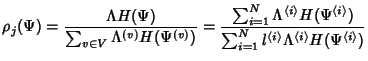
According to [5], the marginal entropy of SNMP data
collected on link can be calculated as:
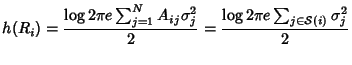 |
(21) |
The joint entropy of SNMP
data collected on link and can be calculated as:
where
 is the -th row vector in routing
matrix is the -th row vector in routing
matrix  and and
 , ,
 and and
 . Therefore . Therefore
where
 is the covariance
coefficient between is the covariance
coefficient between  and and  . The mutual information
between SNMP data on link and link is . The mutual information
between SNMP data on link and link is
which could be small even
if  is close to one. For example, suppose there are is close to one. For example, suppose there are
 flows traversing both link and link . In addition to
those common flows, links and each have their own flows traversing both link and link . In addition to
those common flows, links and each have their own  flows. If we assume all flows are statistically homogeneous, then
we will have
flows. If we assume all flows are statistically homogeneous, then
we will have
 , which indicates and are
highly correlated. However, according to (22), the
mutual information between and is only around , which indicates and are
highly correlated. However, according to (22), the
mutual information between and is only around  bits. This suggests there is not much gain in doing joint
compression of SNMP data.
bits. This suggests there is not much gain in doing joint
compression of SNMP data.
5.2.2 How much information does SNMP contain about traffic matrices?
For the purpose of traffic engineering, it is
important to characterize the traffic demand between all pairs of
network ingress and egress points, or the Traffic Matrix (TM).
Each element in the TM corresponds to the traffic rate of the flow
class which goes from the ingress point to the egress point. Such
information is normally not easy to access. Network operators can
instrument each router to record SNMP data on each link, which is
the sum of traffic rates of all flow classes traversing that link.
It is challenging to infer the TM, equivalently the flow rate
vector, based on the SNMP rate vector [26]. Our
framework provides a way to quantify the amount of information
about a TM that one can obtain from SNMP data.
Essentially, the information content in the flow rate vector (or
TM) is
Since the link rate vector is a linear combination of the flow
rate vector, we will always have
 |
(26) |
Furthermore, under the Gaussian assumption, the information
content in the link rate vector can be calculated as
The gap in (29) is determined by both
the routing matrix and the variance in the traffic rates of
flow classes
 .
Note: For some routing matrices, the rows of
are dependent, i.e., some link rate is a linear
combination of some other link rates. In this case,
contributes no new information to the link rate vector;
consequently, we should only include all independent row
vectors of in (28) to calculate the entropy of
the whole link rate vector. We will illustrate this through an
example in Section5.3.
In this section, we study the entropy rate in SNMP data by
taking into account the temporal correlation in traffic
rate processes. We have observed that the marginal link rate vector
is well characterized as a multivariate Gaussian random variable.
Consequently the link rate vector process over time is a
stationary multivariate Gaussian process with mean .
Note: For some routing matrices, the rows of
are dependent, i.e., some link rate is a linear
combination of some other link rates. In this case,
contributes no new information to the link rate vector;
consequently, we should only include all independent row
vectors of in (28) to calculate the entropy of
the whole link rate vector. We will illustrate this through an
example in Section5.3.
In this section, we study the entropy rate in SNMP data by
taking into account the temporal correlation in traffic
rate processes. We have observed that the marginal link rate vector
is well characterized as a multivariate Gaussian random variable.
Consequently the link rate vector process over time is a
stationary multivariate Gaussian process with mean  given
by (19) and covariance matrix at time lag given
by (19) and covariance matrix at time lag  , ,
 ,
to be determined next. In order to simplify the discussion, we ignore
link delays. These can be accounted for, but at the cost of some obfuscation.
We have
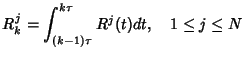
where ,
to be determined next. In order to simplify the discussion, we ignore
link delays. These can be accounted for, but at the cost of some obfuscation.
We have
where
 if and 0 otherwise, and if and 0 otherwise, and
 is the covariance associated with the class rate
process,
. To obtain is the covariance associated with the class rate
process,
. To obtain
 , we return to the
original flow model and recognize that each flow class can be
modeled as an M/G/ , we return to the
original flow model and recognize that each flow class can be
modeled as an M/G/ queue and that we can apply known
results regarding the autocorrelation function of its buffer
occupancy process, [21]. If queue and that we can apply known
results regarding the autocorrelation function of its buffer
occupancy process, [21]. If  denotes the duration
of a class denotes the duration
of a class  flow and flow and  denotes the forward recurrence
time associated with ,
, then
The distribution of is
Suppose that we sample over intervals of length denotes the forward recurrence
time associated with ,
, then
The distribution of is
Suppose that we sample over intervals of length  . Then we
can use a discrete time version of the model where
Note that . Then we
can use a discrete time version of the model where
Note that
 is a discrete time Gaussian
process with mean is a discrete time Gaussian
process with mean
 and covariance approximately equal
to and covariance approximately equal
to
![$ \Gamma^\tau (h) = \Lambda^j E[T^j] \Pr [\hat{T}^j > \vert h\tau\vert]$](img205.png) , ,
 . The discrete time counterparts for the rate
process at the routers can be defined in a similar manner. The
entropy rate of . The discrete time counterparts for the rate
process at the routers can be defined in a similar manner. The
entropy rate of  is given as, [5, Theorem
9.4.1] is given as, [5, Theorem
9.4.1]
where  is the is the  covariance matrix with elements covariance matrix with elements
 , ,
 . Finally, the entropy rate
of the system is . Finally, the entropy rate
of the system is
 . .
5.2.4 SNMP Evaluation
Table 4:
Comparision of SNMP data entropy between model and empirical calculations
| Data Set |
Entropy |
Model |
Empirical |
| SNMP |
 (BB1-out) (BB1-out) |
20.6862 |
20.6700 (max
mse 0.1499) 0.1499) |
| |
(BB2-out) |
20.8895 |
20.8785 (max mse0.1654) |
| |
(C1-in) |
21.0468 |
21.0329 (max mse0.1618) |
| |
(C1-in,BB1-out) |
26.1517 |
26.1254(max mse0.2717) |
| |
(C1-in,BB2-out) |
26.1432 |
26.3078(max mse0.2945) |
|
The SNMP model is derived from the flow model and represents a summary
of flow information. We evaluate the SNMP model by comparing the model
derived entropy with an empirical entropy estimation.
The SNMP data is a per second utilization summarized from our
trace data, instead of real per five minute data collected from
the field. This is done to provide compatibility with
the other monitoring methods. The empirical entropy estimation for
each individual link is based on calculating empirical probability
distribution function from the SNMP data, with a bin size of
50,000 bytes/sec. We use the BUB entropy
estimator [20] with the PDF to derive the entropy.
The BUB estimator does well when the number of available samples
is small compared to the number of bins, as is the case here. It
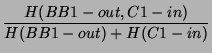
also provides an error bound for the estimation. For joint entropy
such as H(BB1-out, C1-in), we compute the joint probability
distribution of each SNMP data pair at time  : (BB1-out(t),
C1-in(t)), then compute the entropy using the BUB function. In
Table 4 we verify that the entropy of the SNMP data derived from
the Gaussian model indeed matches well with the empirical
calculations. : (BB1-out(t),
C1-in(t)), then compute the entropy using the BUB function. In
Table 4 we verify that the entropy of the SNMP data derived from
the Gaussian model indeed matches well with the empirical
calculations.
5.3 Results
Table 5:
Comparison of entropy calculations in
information gain for different measurement granularity
| Data Set |
Entropy (bits) |
Joint Compression Ratio |
| SNMP |
C1-in 21.0468 |
C1-in and BB1-out 1.0021 |
| |
BB1-out 20.6862 |
C1-in and BB2-out 0.9997 |
| NetFlow |
C1-in 160.8071*697 |
C1-in and BB1-out 0.8597 |
| |
BB1-out 159.6124*1730 |
C1-in and BB2-out 0.8782 |
| Full Trace |
C1-in 706.3773*697 |
C1-in and BB1-out 0.8649 |
| |
BB1-out 736.1722*1730 |
C1-in and BB2-out 0.8702 |
|
We present results on the comparison of the three monitoring
options in terms of quantitative storage difference and
distributed compression savings. The joint compression ratio
indicates whether two links share a strong spatial correlation.
The stronger the links are correlated, the lower the compression
ratio. This is intuitive because when two links share a large
amount of information, the shared information only needs to be
recorded once, hence yielding a large compression savings. In
Table 5, we find that the spatial
correlation is very weak at the SNMP level (compression ratio is
approx. 1), but much stronger at both NetFlow and all packet
monitoring levels (compression ratio is between 0.5 to 0.8702).
This result suggests that there is no need to coordinate SNMP data
gathering at different monitoring points, while coordinated
collection and shared information at all monitoring points can
yield significant savings in terms of storage for widely deployed
NetFlow and all packet monitoring.
Table 5 also shows the information content
comparison among the three monitoring options. SNMP data takes about
21bits to encode per second, while NetFlow takes 74444bits per second,
and all packet monitoring takes 492082bits per second.
Now let's turn to the information gap between SNMP data and actual
flow rate vector as studied in Section5.2.2. For the
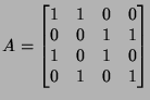
case under study, there are  links and
flow classes between incoming-outgoing link pairs. The routing
matrix is
Row vectors of are dependent:
which means you can obtain the rate on link as
Therefore, links and
flow classes between incoming-outgoing link pairs. The routing
matrix is
Row vectors of are dependent:
which means you can obtain the rate on link as
Therefore,
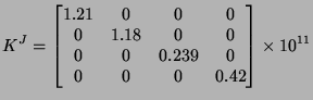
We obtained the rate
variance of each flow classes as:
According to (29), the information content in the
rate vector for all flow classes is
 ; according
to (28), the information content in the rate vector
for all links is ; according
to (28), the information content in the rate vector
for all links is
 . The information gap is . The information gap is
 of the total flow rate information. For this very simple
topology and routing matrix, even if we collect SNMP data on all
incoming and outgoing links, we still cannot fully infer the
traffic rates between all incoming and outgoing pairs. We
conjecture that as the topology and routing gets more complex, the
information gap between the SNMP link rate vector and the flow rate vector
increases, in other words, it becomes more difficult to obtain
the traffic matrix by just looking at the SNMP data. of the total flow rate information. For this very simple
topology and routing matrix, even if we collect SNMP data on all
incoming and outgoing links, we still cannot fully infer the
traffic rates between all incoming and outgoing pairs. We
conjecture that as the topology and routing gets more complex, the
information gap between the SNMP link rate vector and the flow rate vector
increases, in other words, it becomes more difficult to obtain
the traffic matrix by just looking at the SNMP data.
6 Conclusion and Future Work
Our goal in this paper was to put together a framework
in which we could pose, and answer, challenging yet very
practical questions faced by network researchers,
designers, and operators, specifically i) how much
information is included in various types of packet
traces and by how much can we compress those
traces, and ii) how much joint information is included in
traces collected at different points and how can we
take advantage of this joint information?
We obtained a number of interesting results. For example,
we derived an information theoretic bound for the information content in traces
collected at a single monitoring point and therefore were able to
quantify the potential benefit of lossless
compression on those traces.
Not surprisingly, we found that the compression ratio (or information
content) is small in SNMP traces, much higher in NetFLow traces,
and extremely high in full packet traces. This shows that
full packet capture does provide a quantum leap increase in
information about network behavior. However, deploying
full packet capture stations can be expensive. The interesting comparison,
then, is that between the additional cost of full packet capture
(say compared to NetFlow capture), and the additional amount of information
produced by full packet traces (say compared to NetFlow traces).
We are currently working on this problem, but early results seem to indicate
that the increase in information content is proportionally larger
than the increase in cost, suggesting that a full packet monitoring
system gives you "more bang for the buck" (or rather
"more entropy for the buck").
We also found that full packet header traces can be compressed in practice
down to a minimum of 20% of their original size, and that the amount of
compression is a function of the average flow size
traversing that node: the larger the average flow size, the
smaller the compression ratio.
In practice, packet traces are typically captured at multiple
points. Therefore, it is important to understand how much
information content is available in a set of traces, when
that set is considered as a whole (as opposed to as a
set of independent traces). This is turn is crucial to
tackle further problems such as how many monitoring stations
to set up (there might be a point of diminishing returns
at which additional stations do not bring in enough
"fresh" new information) and how to process and analyze
those correlated data traces.
Using our framework, we find
that joint coding or compression of traces further reduces
the marginally compressed traces at the individual monitors. Specifically,
the joint compression ratio (or equivalently,
the additional compression benefit brought by joint coding of
traces) is low for SNMP or byte/packet count traces, higher for NetFlow
or flow-level traces, and significantly higher for packet-level traces.
This means, for example, that joint coding would be very
useful for full packet trace data (and to a lesser extent for NetFlow
data) collected from different monitoring
points and sent back to a NOC or central analysis station.
We are now working on extending the work in this paper to
joint coding techniques for large scale backbone and wireless
networks.
- 1
-
https://dag.cs.waikato.ac.nz/.
- 2
-
https://www.cisco.com/warp/public/732/tech/netflow.
Cisco NetFlow.
- 3
-
CHOI, B.-Y., AND BHATTACHARYYA, S.
On the accuracy and overhead of cisco sampled netflow.
In Sigmetrics Workshop on Large Scale Network Inference (LSNI):
Methods, Validation, and Applications (June 2005).
- 4
-
CHOU, J., PETROVIC, D., AND RAMCHANDRAN, K.
A distributed and adaptive signal processing approach to reducing
energy consumption in sensor networks.
In IEEE Infocom 2003 (April 2003).
- 5
-
COVER, T. A., AND THOMAS, J. A.
Information theory.
John Wiley & Sons, Inc., 1991.
- 6
-
CRISTESCU, R., BEFERULL-LOZANO, B., AND VETTERLI, M.
On network correlated data gathering.
In INFOCOM (Hong Kong, 2004).
- 7
-
DUFFIELD, N., AND GROSSGLAUSER, M.
Trajectory sampling with unreliable reporting.
In IEEE Infocom (March 2004).
- 8
-
DUFFIELD, N., LEWIS, J. T., O'CONNELL, N., RUSSELL, R., AND TOOMEY, F.
Entropy of atm traffic streams: A tool for estimating qos parameters.
IEEE JSAC, 13 (1995), 981-990.
- 9
-
DUFFIELD, N., LUND, C., AND THORUP, M.
Properties and prediction of flow statistics from sampled packet
streams.
In IMW '02: Proceedings of the 2nd ACM SIGCOMM Workshop on
Internet measurment (New York, NY, USA, 2002), ACM Press, pp. 159-171.
- 10
-
FRALEIGH, C., MOON, S., LYLES, B., COTTON, C., KHAN, M., MOLL, D.,
ROCKELL, R., SEELY, T., AND DIOT, C.
Packet-level traffic measurements from the sprint IP backbone.
IEEE Network (2003).
- 11
-
HOHN, N., AND VEITCH, D.
Inverting sampled traffic.
In ACM/SIGCOMM Internet Measurement Conference (November
2003).
- 12
-
HOHN, N., VEITCH, D., AND ABRY, P.
Cluster process, a natural language for network traffic.
In IEEE Transactions on Signal Processing, Special Issue on
Signal Processing in Networking (August 2003), vol. 51, pp. 2229-2244.
- 13
-
HOHN, N., VEITCH, D., PAPAGIANNAKI, K., AND DIOT, C.
Bridging router performance and queuing theory.
In ACM Sigmetrics (New York, 2004).
- 14
-
IANNACCONE, G., DIOT, C., GRAHAM, I., AND MCKEOWN, N.
Monitoring very high speed links.
In Proceedings of ACM Internet Measurement Workshop (November
2001).
- 15
-
K. MCCLOGHRIE, M. T. R.
Rfc 1213.
- 16
-
LEE, W., AND XIANG, D.
Information-theoretic measures for anomaly detection.
In IEEE Symposium on Security and Privacy (2001).
- 17
-
LELAND, W., TAQQU, M., WILLINGER, W., AND WILSON, D. V.
On the self-similar nature of ethernet traffic.
IEEE/ACM Transactions on Networking 2, 1 (February 1994).
- 18
-
LIU, X., AND SRIKANT, R.
An information-theoretic view of connectivity in wireless sensor
networks.
In IEEE SECON (Conference on Sensor Networks and Adhoc
Communications and Networks) (2004).
- 19
-
LIU, Y., TOWSLEY, D., WENG, J., AND GOECKEL, D.
An information theoretic approach to network trace compression.
Tech. Rep. UMASS CMPSCI 05-03, University of Massachusetts, Amherst,
2004.
- 20
-
PANINSKI, L.
Estimation of entropy and mutual information.
Neural Computation 15, 1191-1254 (2003).
- 21
-
PARULEKAR, M., AND MAKOWSKI, A.
TEX2HTML_WRAP_INLINE$M/G/&infin#infty;$ input processes: A versatile
class of models for network traffic.
In Proceedings of INFOCOM (1997).
- 22
-
PATTEM, S., KRISHNAMACHARI, B., AND GOVINDAN, R.
The impact of spatial correlation on routing with compression in
wireless sensor networks.
In IPSN'04: Proceedings of the third international symposium on
Information processing in sensor networks (2004), pp. 28-35.
- 23
-
PEUHKURI, M.
A method to compress and anonymize packet traces.
In Proceedings of ACM Internet Measurement Workshop (November
2001).
- 24
-
PLOTKIN, N., AND ROCHE, C.
The entropy of cell streams as a traffic descriptor in atm networks.
In IFIP Performance of Communication Networks (October 1995).
- 25
-
ZHANG, Y., DUFFIELD, N., PAXSON, V., AND SHENKER, S.
On the constancy of internet path properties.
In Proc. ACM SIGCOMM Internet Measurement Workshop (2001).
- 26
-
ZHANG, Y., ROUGHAN, M., LUND, C., AND DONOHO, D.
An information-theoretic approach to traffic matrix estimation.
In ACM SIGCOMM (August 2003).
An Information-theoretic Approach to Network Monitoring and Measurement
This document was generated using the
LaTeX2HTML translator Version 2002 (1.62)
Copyright © 1993, 1994, 1995, 1996,
Nikos Drakos,
Computer Based Learning Unit, University of Leeds.
Copyright © 1997, 1998, 1999,
Ross Moore,
Mathematics Department, Macquarie University, Sydney.
The command line arguments were:
latex2html -split 0 -show_section_numbers -local_icons imc.tex
The translation was initiated by Yong Liu on 2005-08-09
Yong Liu
2005-08-09
|

![$\displaystyle \sum_{j\in[0,N]} h(R^j)$](img180.png)
![$\displaystyle \sum_{j\in[0,N]} \frac{1}{2} \log 2\pi e \sigma_j^2.$](img181.png)
![$\displaystyle \Pr [\hat{T}^j > h] = \frac{1}{E[T^j] }\int_h^\infty \Pr [T^j > x] dx, \quad h\geq 0 $](img200.png)