Context-based Routing: Techniques, Applications and Experience
Saumitra Das1, Yunnan Wu2, Ranveer Chandra2, Y. Charlie Hu1 |
Abstract:Routing protocols in multi-hop networks typically find low cost paths by modeling the cost of a path as the sum of the costs on the constituting links. However, the insufficiency of this approach becomes more apparent as new lower layer technologies are incorporated. For instance, to maximize the benefit of multiple radios, ideally we should use routes that contain low interference among the constituting links. Similarly, to maximize the benefit of network coding, we should ideally use routes that create more coding opportunities. Both of these are difficult to accomplish within the conventional routing framework because therein the links are examined in isolation of each other, whereas the nature of the problem involves interdependencies among the links.
This paper aims at revealing a unifying framework for routing in the presence of inherent link interdependencies, which we call “context-based routing". Through the case studies of two concrete application scenarios in wireless networks, network coding–aware routing and self-interference aware routing in multi-radio systems, we highlight the common key pillars for context-based routing and their interplay: a context-based path metric and a route selection method. We implement context-based routing protocols in Windows XP and Linux and evaluate them in detail. Experiments conducted on 2 testbeds demonstrate significant throughput gains.
Routing in wireless mesh networks is a well studied problem. A common practice is to model the cost of a path as the sum of the costs on the constituting links, where the link cost reflects the link quality, e.g., the per-hop round-trip time (RTT) [1], the expected transmission count (ETX) [2], and the expected transmission time (ETT) [4]). Routing then aims at finding the path offering the lowest total cost. However, the inadequacy of this widely used approach becomes evident as new lower layer technologies appear.
For example, a promising technique for improving the capacity of wireless mesh networks is to use multiple radios. With multiple radios, more concurrent communications can be packed in spectrum, space and time. To maximize the benefit of multiple radios, ideally we should use routes that contain low interference among the constituting links. Another example is link layer network coding, a recent advance [6] that exploits the broadcast nature of the wireless medium. Network coding, on its own, can improve the link layer efficiency. The gain of this technique, however, critically depends on the traffic pattern in the network, and hence the routing decisions. To maximize the benefit of network coding, ideally we should use routes that create more mixing opportunities. In these scenarios, the conventional routing framework does not perform well because therein the links are examined in isolation of each other. To fully leverage the lower layer advances, we need advanced routing techniques that can properly model the inherent interdependencies of the links in order to identify good routes.
Related Work: For multi-radio systems, some progress has been made in selecting interference aware routes. The WCETT [4] (Weighted Cumulative Expected Transmission Time) metric penalizes a path that uses the same channel multiple times, thus modeling link interference to some extent. However, WCETT assumes that all links on a route that use the same channel interfere, which does not incorporate the phenomenon of spatial reuse and may miss high-throughput routes that reuse channels carefully at links sufficiently apart (see Figure 4). Moreover, [4] uses Dijkstra's shortest path algorithm. Although Dijkstra's algorithm is optimal for the conventional path metric, i.e. a sum of link costs, it is not optimal for WCETT. Another proposal for interference aware routing is the MIC (metric of interference and channel-switching) metric [13, 14] and the authors also showed how to find the optimal route under this metric in polynomial time. However, to ensure finding the optimal path in polynomial time, the metric is forced with some constraints (decomposability, fixed memory) that may not match well with the nature of the underlying link interdependencies. This can cause issues in modeling the costs of routes (see Figure 5), and as a result, the path found can be inefficient.
Network coding–aware routing has been studied in [8, 11] from theoretical perspectives. These papers presented theoretical, flow-based formulations for computing the throughput with network coding and network coding–aware routing, assuming centralized control in routing and scheduling. To characterize the gain of network coding, these theoretical studies showed that it is necessary to examine two consecutive hops jointly, because of the link interdependency.
Overview: These previous studies have offered insight in dealing with link interdependencies. This paper aims at revealing a unifying framework for routing under inherent link interdependencies, which we call “context-based routing". We proceed by studying two concrete application scenarios: network coding–aware routing, and self-interference aware routing. Through these case studies, we highlight the common key pillars for context-based routing and their interplay, and provide a more systematic treatment of these pillars. In particular, we show how to overcome the shortcomings of the aforementioned approaches for self-interference aware routing in multi-radio systems and also apply the techniques more generally to other scenarios.
The first pillar is the concept of context-based link metrics, which can model the interactions among different links in a route. Context refers to examining the cost of each link based on what links are used prior to the current link. Having such context allows us to evaluate the “goodness” of routes by considering the impact of the links on each other. More specifically, the conditional link costs allow us to conveniently characterize effects such as: (i) the self-interference caused by other links of the same flow, and (ii) the reduction of channel resource consumption due to the use of network coding.
The second pillar is an optimized route selection module, which can search for good paths under a context-based link metric. The interdependencies among the links in a context-based link metric make it challenging to search for a good path. To make things worse, sometimes the context-based link metric is by nature globally coupled, meaning that the cost of a link can depend on as far as the first link. We propose a general context-based path pruning method (CPP). To model the context of a partial path while avoiding the exponential growth in the number of partial paths, CPP maintains a set of paths that reach each node, corresponding to different local contexts. Each local context can be viewed as a concise summary of the dominating history of all the partial paths that end with that local context1, based on the observation that older history usually has less impact on the future. The best path under each local context is maintained and considered further for possible expansion into a source–destination path.
The use of local contexts in path pruning is synergistic with the use of contexts in cost modeling. Together, these two pillars form a context-based routing protocol (CRP), which outperforms existing approaches in scenarios where modeling link-interdependencies is critical. The essence and key technical contribution of CRP lies in (i) properly modeling the link interdependencies (via the context-based metric) and (ii) handling the ensuing algorithmic challenges in route optimization (via CPP).
We have implemented CRP on Windows XP and Linux. While our current implementation assumes link-state routing, other generalizations are also possible. Our evaluations show that CRP provides TCP throughput gains up to 130% and on average around 50% over state-of-the-art approaches for multi-radio networks and gains of up to 70% over state-of-the-art approaches for wireless network coding.
The rest of the paper is organized as follows: Section 2 defines context-based routing metrics and their application to two scenarios. Section 3 describes a general technique of context-based path pruning for finding routes under context-based routing metrics. Section 4 evaluates the performance of the overall context-based routing solution. Finally, Section 5 concludes the paper.
In this section, we discuss what context-based routing metrics are and how they help in modeling link interdependencies. The common defining feature of context-based metrics is that the cost of a link is context-dependent (dependent on what links are already part of the route). To make things concrete, we consider two specific systems: multi-radio multi-channel networks and single-radio networks equipped with network coding and show how context-based metrics can better match the nature of the problems.
In this section, we define a context-based metric that can help make better routing decisions in wireless networks equipped with network coding.
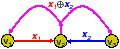
In network coding, a node is allowed to generate output data by mixing (i.e., computing certain functions of) its received data. The broadcast property of the wireless medium renders network coding particularly useful. Consider nodes v1, v2, v3 on a line, as illustrated in Figure 1. Suppose v1 wants to send packet x1 to v3 via v2 and v3 wants to send packet x2 to v1 via v2. A conventional solution would require 4 transmissions in the air (Figure 1(a)); using network coding, this can be done using 3 transmissions (Figure 1(b)) [12]. It is not hard to generalize Figure 1 to a chain of nodes. For packet exchanges between two wireless nodes along a line, the consumed channel resource could potentially be halved.
(a)
(b)
Katti et al. [6] recently presented a framework for network coding in wireless networks, in which each node snoops on the medium and buffers packets it heard. A node also informs its neighbors which packets it has overheard. This allows nodes to know roughly what packets are available at each neighbor (i.e., “who has what?"). Knowing “who has what" in the neighborhood, a node examines its pending outgoing packets and decides how to form output mixture packets, with the objective of most efficiently utilizing the medium. These prior studies result in a link layer enhancement scheme in the networking stack. The network coding engine sits above the MAC layer (e.g., 802.11) and below the network layer. Given the routing decisions, the network coding engine tries to identify mixing opportunities. The gain of this technique, however, critically depends on the traffic pattern in the network. This motivates the following question: Can intelligent routing decisions maximize the benefits offered by network coding?
A natural thought is to modify the link metrics to account for the effect of network coding in reducing transmissions. This, however, is not straightforward. Consider the example setting illustrated in Figure 2. There are two long-term flows in the network, v3 → v2 → v1 and v1→ v4 → v7. We want to find a good routing path from v1 to v9. Due to the existence of the network coding engine, the route v1 → v2 → v3 → v6 → v9 is a good solution because the packets belonging to this new flow can be mixed with the packets belonging to the opposite flow v3 → v2 → v1, resulting in improved resource efficiency. To encourage using such a route, can link v2→ v3 announce a lower cost? There are some issues in doing so, because a packet from v5 that traverses v2→ v3 can not share a ride with a packet from v3 that traverses v2→ v1, although a packet from v1 that traverses v2→ v3 can.
Thus, in the presence of the network coding engine, assessing the channel resource incurred by a packet transmission requires some context information about where the packet arrives from. For example, we can say that given the current traffic condition, the cost for sending a packet from v2 to v3, that previously arrives from v1, is smaller. The key observation here is the need to define link cost based on some context information2. Specifically, for this application, we model the cost of a path P=v0→ v1 → … → vk as the sum of the conditional costs on the links:
|
Here cost(b→ c| a→ b) denotes the cost of sending a packet from b to c, conditioned on that the packet arrived from a. The central issue is to properly define the link costs and compute them. Let us begin by reviewing a conventional (unconditional) link metric. A popular link quality metric in the literature is the expected transmission count (ETX) [2]. This metric estimates the number of transmissions, including retransmissions, needed to send a unicast packet across a link. The ETX metric is a characterization of the amount of resource consumed by a packet transmission.
We now describe how to define a conditional link metric to model the resource saving due to network coding. With network coding, several packets may share a ride in the air. Naturally, the passengers can share the airfare. In effect, each participating source packet is getting a discount. Such a discount, however, cannot be accurately modeled by an unconditional metric such as ETX, because the applicability of the discount depends on the previous hop of the packet. We propose a conditional link metric called the expected resource consumption (ERC), which models the cost saving due to network coding. Consider a packet sent in the air. If it is a mixture of k source packets, then each ingredient source packet is charged 1/k the resource consumed by the packet transmission. The resource consumed could be measured in terms of, e.g., air time, or consumed energy.
We now explain how to concretely compute the ERC. Each node maintains a WireInfoTable. Each row of the table contains the measured statistics about a wire. A wire is a virtual link that connects an incoming and outgoing link from a node (connected the past and future hop), e.g. ei,j→ ej,k, which crosses the current node vj. A cost of a wire ei,j→ ej,k represents the conditional cost cost(j→ k| i→ j). The packets forwarded by the current node can be classified into categories associated with the wires. A packet that is received along ei,j and sent along ej,k falls into the category “ei,j→ ej,k”. For each wire category, we collect the total number of packets sent and the total resource consumed in a sliding time window. The total resource consumption is obtained by adding the resource consumption for each sent packet. A simple charging model is used in our current implementation. For example, if a source packet across wire ei,j→ ej,k is sent in a mixture of 3 packets, we set the resource consumption of this source packet as 1/3 of the ETX of link ej,k. (We could also use ETT [4] in lieu of ETX.)
To implement the sliding window computation efficiently, we quantize the time axis into discrete slots of equal length. We use a sliding window of N slots. For each wire, we maintain a circular buffer of N bins; at any time, one of the N bins is active. At the start of each slot, we shift the active bin pointer once and clear the statistics in the new active bin. Each time a packet is transmitted in the air, we update the statistics in the current active bin accordingly. We use N=10 slots, each of length 0.5s.
To evaluate the conditional link metric for a certain wire ei,j→ ej,k, we first obtain the ERC for each slot, say n, as: ercn := Resource consumed by pkts sent in slot n/# of packets sent in slot n. Then we compute the ERC for the wire as the weighted average of the ERCs for the slots:
|
Here the parameter α is the forgetting factor for old observations. Older observations receive lower weights. In the simulations, we use α = 0.8.
The above measurement method generates an estimate of the current ERC, which is the ERC seen by a flow whose packets are currently being mixed. To bootstrap new flows to favor routes that expose mixing opportunities, in addition to the current ERC, we also collect another statistic called the marginal ERC. The marginal ERC reflects the potential new ERC, i.e., with discount, for a wire if a new flow decides to use a route that contains that wire. A flow decides on its initial route or switches to a new route based on the marginal ERC. Afterwards, the current ERC for each wire in the chosen route is updated and is used instead. If the existing flows already use up most of the mixing opportunities, then the marginal ERC will not have a high discount. Both the current ERC and the marginal ERC are reported. To compute the marginal ERC, a simple rule is applied in our current implementation. Specifically, for a wire eij→ ejk in a given time slot, we examine the number of unmixed packets y in the reverse wire ekj→ eji. If y≥ 25, then we set the marginal ERC as 0.75 of the ETX (25% discount); otherwise, we set the marginal ERC as the ETX (no discount).
ERC takes the traffic load into account. Could this cause oscillation in the routing decisions? The advertised discounts are conditional by definition; hence they typically only apply to a specific set of flows (those that can be mixed with the existing flows at a node). For example, node v2 in Figure 2 might advertise a smaller conditional cost, cost(v2→ v3| v1→ v2) < cost(v2→ v3), to reflect that traffic going v1 to v2 and then v3 can be mixed with the existing flows. Such conditional discounts can only be taken advantage by flows that uses the segment v1→ v2→ v3. There is incentive for this specific set of flows to route in a certain cooperative manner that are mutually beneficial. Presumably, if the flows try such a mutually beneficial arrangement for some time, they will confirm the discounts and tend to stay in the arrangement. To prevent potential route oscillations, we require each flow to stay for at least Thold duration after each route change, where Thold is a random variable. The randomization of the mandatory route holding time Thold is used to avoid flows from changing routes at the same time. In addition, after the mandatory route holding duration, the node switches to a new route only if the new route offers a noticeably smaller total cost.
In summary, using context conveniently represents paths that benefit from network coding. We now show another example of a context-based metric for networks with multiple-radios.
In this section, we define a context-based metric that can help make better routing decisions in wireless networks equipped with multiple radios.
Consider a multi-hop wireless network equipped with multiple radios. Similar to [4], we assume each radio is tuned to a fixed channel for an extended duration; a route specifies the interfaces to be traversed. We define a context-based SIM (self-interference aware) metric, as a weighted sum of two terms:
|
where ek is the k-th edge along the path P.
The first term is the sum of the expected transmission time along the route. The ETT [4] metric aims at estimating the average transmission time for sending a unit amount of data. It is defined as: ETT =Δ PktSize·ETX/Link Bit-Rate. ETX [2] is computed as ETX=Δ 1/(1−p), where p is the probability that a single packet transmission over link e is not successful. The link bit-rate can be measured by the technique of packet pairs and this method can produce sufficiently accurate estimates of link bandwidths [3].
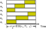
The second term caculates the estimated service interval (ESI) at the bottleneck link, which reflects how fast the route can send packets in the absence of contending traffic. Note that the max operation is used here instead of the sum operation. This can be explained by a pipeline analogy. In a pipeline system consisting of several processing stages, the long term throughput is determined by that of the bottleneck stage, rather than the average throughput of the stages. Sending packets along a wireless route is similar. The long term throughput of a flow is determined by that of the bottleneck link.
The ESI of a link is defined as:
|
Here Pk−1 is the partial path with k−1 links, and pjk is a binary number that reflects whether ej and ek interfere. Characterizing the interference relations among the links is itself a research challenge. For instance, one method is to make use of actual interference measurement; see, e.g., Padhye et al. [9] and the references therein. Consider two links, A→ B and C→ D, using the same channel. As suggested in [9], for 802.11 networks, the primary forms of interference are four cases: (i) C can sense A's transmission via physical or virtual carrier sensing, and hence refrains from accessing the medium, (ii) A can sense C's transmission, (iii) transmissions of A and C collide in D, (iv) transmissions of A and C collide in B. Based on this, we adopt a simplified approach in the experiments of this paper. We treat the two links as interfering if A has a link to C or D with sufficiently good quality, or C has a link to A or B with sufficiently good quality.
The ESI expression (4) leaves out the interference caused by other contending traffic. This is a simplification in modeling. The ESI expression (4) considers the self-interference from the previous hops of the route, by adding up the expected transmission times of the previous links. The intuition is that the packets at the link needs to share the channel with the interfering links on the route. One might ask why we do not add the ETTs from the subsequent links on the path, even though both previous and subsequent links can create interference. The following theorem provides an answer.
Proof: Under the assumptions in the claim, finding the optimal end-to-end throughput essentially amounts to finding an optimal interference-free scheduling of the uses of the constituting links. If we can schedule each link to transfer B bits in T seconds, then the throughput B/T can be achieved. It is well known that this problem can be viewed as a continuous version of the graph coloring problem on the conflict graph.
In greedy coloring algorithms, nodes in a graph are visited one by one. Each node tries to reuse some existing colors if possible. If not, the node selects a new color. With this procedure, it is easy to see that the graph can be colored in Δ(U)+1 colors, where Δ(U) is the maximum degree of a vertex. Notice that the greedy coloring algorithm always look at the already colored nodes, but not future nodes. Hence in fact the upper-bound can be tightened to one plus the maximum number of already-colored neighbors for the nodes. We now apply a greedy-coloring like algorithm for scheduling the links on a route. This is illustrated in Figure 3 for a path with 6 links. We visit the links on the route sequentially, from the first hop to the last hop. For each link ek, find one or more intervals with a total length of ETT(ek) that do not cause interference with any of the previous k−1 links. Similar to greedy coloring, when assigning the intervals to a link, we only need to examine the previous links, but not future links. With this greedy scheduling process, we can finish the assignment in a total duration of maxkESI(ek|Pk−1). If we repeat this scheduling pattern for a sufficiently long time, then we can deliver one packet end to end every maxkESI(ek|Pk−1) (sec). Hence the throughput is achievable.
The above theorem shows that the bottleneck ESI corresponds to a theoretically achievable throughput. Conversely, if a link ek interferes with a set F of previous links, then typically links in F∪ {ek} would be expected to mutually interfere (hence forming a clique in the conflict graph). If that indeed is the case, then we cannot deliver more than one packet end to end every maxkESI(ek|Pk−1) (sec). This argument shows that the maximum throughput is roughly around 1/maxkESI(ek|Pk−1).
The bottleneck ESI models self-interference. The previously introduced metrics, WCETT and MIC, also consider self-interference. We now compare the proposed SIM metric with WCETT and MIC.
The WCETT metric proposed by Draves et al. [4] is defined as:
|
Here ek denotes the k-th hop on the path P and β is a weighting factor between 0 and 1. The WCETT metric is a weighted sum of two terms. The first term is the sum of the ETT along the path. The second term aims at capturing the effect of self-interference. A path that uses a certain channel multiple times will be penalized.
(a)
(b)
(c)
Figure 4: (a) Chain topology. Each node has 3 radios on orthogonal channels 1, 2, 3. (b) Route selected by using the WCETT metric. (c) Route selected by using the SIM metric.
Although WCETT considers self-interference, it has some drawbacks. Consider the following example. Figure 4(a) shows a chain topology, where each node has three radios tuned to orthogonal channels 1,2,3. We assume two links within 2 hops interfere with each other if they are assigned the same channel. We further assume all links have similar quality. An ideal route in this setting is then a route that alternates among the three channels, such as the one illustrated by Figure 4(c), because it can completely avoid self-interference. Figure 4(b) shows a possible solution returned by WCETT. This route suffers from primary interference as well as secondary interference. This can be explained by the way WCETT models self-interference. From (5), it is seen that WCETT views a path as a set of links. In this example, it tries to maximize channel diversity by balancing the number of channels used on the path. Thus the path in Figure 4(b) and the path in Figure 4(c) appear equally good under WCETT.
In essence, WCETT takes a pessimistic interference model that all links on the same channel in the route interfere with each other. Indeed, if we use this interference model, then SIM reduces to WCETT. The proposed SIM metric models self-interference can differentiate different ordering of the links in the path and find the optimal path for this example. The benefit is that SIM potentially allows better channel reuse.
Another self-interference aware metric is the metric of interference and channel-switching (MIC), proposed by Yang et al. [13, 14]. The MIC metric is defined as:
|
Here α>0 is a weighting factor to balance the two terms. In (7), Nk is the number of neighbors in the network that interferes with the transmission of link ek. The IRU (interference-aware resource usage) term aims at reflecting the inter-flow interference. A link that interferes with more neighbors will be penalized. The CSC (channel-switching cost) aims at reflecting the self-interference, since it penalizes consecutive uses of the same channel.
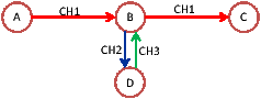
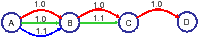
The total CSC term (8) in the MIC metric models the self-interference by considering the immediate previous hop. As an extension, the authors also considered the extension of the MIC metric to model self-interference for more than one hops [14]. However, a potential limitation with the MIC metric and its multi-hop extension is that it has a fixed limited memory span. Consider the example in Figure 5. Suppose the links between nodes A and B have very low costs. Under the MIC metric, it is possible that the route A→ B→ D→ B → C has a lower cost than the route A→ B→ C. Since the path is selected by optimizing the metric, it is unclear whether the MIC metric can rule out the possibility of selecting a pathological path, which has self-interference that are not modeled in the MIC expression.
Compared with the MIC metric, the SIM metric considers the possible interference with all previous hops. This avoids the pathological case as shown in Figure 5. In addition, whereas the link CSCs are summed up in (6), SIM uses the maximum ESI. The use of the maximum operation can better reflect the fact that the throughput is determined by the bottleneck link.
The previous section showed two concrete examples of how context helps in making routing metrics more powerful. After defining a good context-based path metric, the subsequent challenge is to find the optimal (or near-optimal) route under the path metric. A context-based routing protocol needs both a context-based metric and a way to find good paths under such metrics. In this section, we develop such a path finding method called CPP (Context-based Path Pruning) that can find paths under any generic context-based metric. As a starting point, we first consider a link state routing framework. In link state routing, each router measures the cost to each of its neighbors, constructs a packet including these measurements, sends it to all other routers, and computes the shortest paths locally. Hence for link state routing, what is needed is a centralized algorithm for computing the shortest paths. The CPP method will be explained as a centralized algorithm. But we note that it can also be applied in some distributed settings, such as distance vector protocols and on-demand route discovery; these extensions are omitted in the interest of space.
Let us begin by reviewing the (simpler) problem of finding the optimal path under a path metric where each link has a nonnegative cost and the cost of a path is the sum of the costs of the constituting links. This problem is well understood. For example, the classical shortest path algorithm by Dijkstra can be applied to find the optimal path with complexity O(|V|2), where |V| denotes the number of nodes in the network. Dijkstra's algorithm maintains upper-bound labels f(v) on the lengths of minimum-cost s–v paths3 for all v∈ V. The label of each node is either temporary or permanent, through the execution of the algorithm. At each iteration, a temporary label with the least total cost is made permanent and the remaining temporary labels are updated. Specifically, if v* has the minimum total cost among the temporary nodes, then we update the cost of every other temporary node w as:
|
Dijkstra's algorithm operates on an optimality principle: The shortest path from s to t via v is the shortest path from s to v concatenated with the shortest path from v to t. Thus, each node only needs to remember the cost of the best s–v path. Such optimality principle no longer holds for metrics such as SIM, ERC or WCETT; for such metrics, an s–v path P1 may have a larger cost than an s–v path P2 but may eventually lead to a lower cost toward the final destination node t.
We propose a context-based path pruning (CPP) technique as a heuristic method for optimizing a context-based metric. To model the potential impact of past hops on future hops, we maintain a set of paths that reach each node v, instead of a single s–v path with minimum cost. A natural question is: How many paths should we store at each node as we search for a good s–t path? Storing all paths would apparently result in an exponential complexity. To keep the complexity manageable, we maintain only a small subset of s–v paths at a node v; the size of the subset is constrained by the affordable computation complexity. Ideally we want this small set to cover all “promising" s–v paths, which have the potential of leading to an optimal s–t path. How do we select this set then? Consider dividing an s–t path into three parts as:
|
A good route in a wireless mesh network typically moves in the direction toward the destination. If the second part P2 is sufficiently long, typically the first segment sP1⇝u would be well separated from the third segment v P3⇝ t; as a result, there would not be a strong interdependency between the first and the third segment. In other words, the link interdependencies of a wireless route are typically localized in nature. This observation motivates us to organize the memory at each node according to several local contexts. As a concrete example, we can define the local context of an s–v path as the sequence of links in the last l hops, where l is a predetermined parameter. Under this definition, if P2 in (10) is l-link long, then the local context of the s–v path sP1⇝u P2⇝ v is the sub-path P2. The s–v paths with the same local contexts are grouped together. During the execution of the proposed algorithm, node v always keeps only one s–v path under each local context, i.e., the minimum cost one found so far in the algorithm execution. The algorithm works by examining the paths stored at the nodes and considering them for potential expansion into an s–t path.
In the above we have given a concrete example definition of the local context, where the local context of an s–v path is defined as the sequence of links in the last l hops, where l is a predetermined parameter. For the scenario of network coding–aware routing, we use this definition with l=2. As another concrete example, we can define the local context of an s–v path as the the sequence of channels taken by the links in the last l hops. This definition is useful for the scenario of self-interference aware routing. In general, the definition of local contexts is problem specific.
Algorithm 1 A Context-based Path Pruning Method
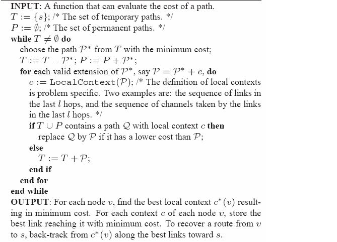
More formally, Algorithm 1 shows a Dijkstra-style instantiation of the CPP method. We maintain a set T of temporary paths and a set P of permanent paths4. In each step, we choose the temporary path with minimum cost. Such a path, say P*, is made permanent. Then we consider the possible ways of extending P* toward an s–t path. For each extension P=P* + e, we determine its local context and search for a path with the same local context in T and P. If a path with the same local context already exists, then such existing path is compared with P and the winner is retained. If a path with the same local context does not exist, then P is added to T.
There is an alternative way to understand the CPP method. For each physical node v, introduce one vertex vc for each local context c applicable to v and interconnect the vertices according to original connectivity. Denote such a context-expanded graph by Gc. We can interpret Algorithm 1 as applying a revised version of the Dijkstra's algorithm to the expanded graph Gc. More specifically, since here the path metric is not decomposable, the cost update step (9) needs to be revised. Instead of using (9), node v* first reconstructs the current best path from the source, say s⇝Pv*. Then each neighbor node w of v* is updated using the following path-based update rule:
|
where cost(·) returns the path metric.
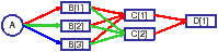
We now start from the network in Figure 6 and show how to construct context-expanded graphs for it. Here there are there orthogonal links from A to B, two links from B to C, and one link from B to C. The ETT metrics for the links are shown on the links. Consider β=0.5 and the SIM metric (3). In this example, Dijkstra's algorithm using the path-based update rule (11) will return A—→CH1B—→CH2C—→CH1D, with a total cost of 0.5*(1.0+1.1+1.0)+0.5*max{1.0+1.0,1.1}=2.55.
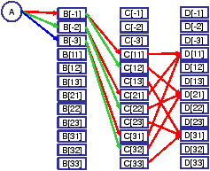
Figure 7 shows the expanded graph for the case the local contexts are defined by the previous hop's channel ID. Taking the original node B as an example, there are three nodes in Gc, which are associated with three channels to reach B. To connect Algorithm 1 with running Dijkstra's algorithm using the path-based update rule (11) over the expanded graph, we can view each node as storing the optimal path reaching it from the source; the optimal path can be obtained by backtracking along the best links that reach each node. In this case, the optimal route found is A—→CH2B—→CH1C—→CH1D, with a total cost of 0.5*(1.0+1.0+1.0)+0.5*max{1.0+1.0,1.0}=2.5.
If the local contexts are defined by the previous two hops' channel IDs, then the resulting expanded graph would be the one shown in Figure 8(c). This will yield the optimal route A—→CH3B—→CH2C—→CH1D, with a total cost of 0.5*(1.1+1.1+1.0)+0.5*max{1.1,1.1,1.0}=2.1.
Handling the ERC metric is simpler for CPP since ERC simple has one-hop of memory. Thus the local context is simply defined as the previous hop on which the packet arrived instead of specifying the channel. This shows that CPP is a generic technique which can be used for many context-based metrics by defining the local contexts in accordance with the definition of the metric being used.
If the path metric indeed has a fixed memory span (say, l hops) such as in ERC, then CPP with the local context defined by the l-hop links is guaranteed to find a route that minimizes the given path metric (because no pruning step is suboptimal). In our case, the SIM path metric has a memory span that could potentially involve the entire path history. Even if the path metric has a longer memory span than the length of the local contexts, the CPP method can still be applied as an effective heuristic method.
Yang et al. [13, 14] proposed a method for finding the optimal route under the MIC metric (6) and its multi-hop generalization in polynomial time complexity. The method hinges upon the fact that the path metric is decomposable into a sum of link costs, where the cost of a link depends only a fixed number of previous hops; in other words, the path metric is additive and has a fixed memory span. In [13, 14], a virtual graph is constructed, by introducing virtual vertices and edges to represent different states; each edge has an associated cost. Then finding an optimal route under the decomposable, finite-memory metric in the original problem becomes the problem of finding an optimal path in the virtual graph under a memoryless metric, where the cost of a path is simply the sum of the costs of the constituting edges. Therefore, for the additive path metric with a fixed memory span, the optimal solution can be found in polynomial time.
In comparison, the CPP method is applicable for all path metrics, not only when the path metric is decomposable and has finite memory. A key feature of the CPP method is the explicit differentiation of two memories: the path metric's memory and the local context's memory. The path metric's memory can be chosen to best model the path cost. For instance, the path metric based on ERC has 2-hop memory; the SIM path metric has global memory. However, the local context's memory will be chosen based on complexity. These two memories need not be equal length. When the path metric is decomposable and has finite memory, CPP can also find the optimal answer, by using a local context with the same memory length as the path metric. When the path metric is not decomposable, CPP can still be used, as a heuristic method. This comes from the fact that CPP operates by always examining the partial-paths from s and applying the path metric to evaluate their costs, which is apparent from Algorithm 1, as well as the path-based update rule in (11). Observe also that the edges in Figures 7 and 8 do not have associated costs, in contrast to the virtual graph in [13, 14]. Although the local context used in CPP only has limited information about the path history, the path metric has the information of the complete path and can properly take into account any local or global link interdependency. This mix of “local" memory and “global" path evaluation metric is a distinct feature of the CPP method, rendering it generally applicable and efficient.
As we mentioned earlier, Algorithm 1 can be essentially viewed as applying Dijkstra's algorithm with the path-based update rule (11) over the expanded graph. Note though that in Algorithm 1, the involved vertices and links are constructed on the fly, without explicitly maintaining the expanded graph. Due to the connection between Algorithm 1 and Dijkstra's algorithm, we can easily conclude that the time complexity of the Algorithm 1 is O(C2), where C is the total number of local contexts at all nodes. If we define the local context of a path as the sequence of channels taken by the links in the last l hops, then C is upper-bounded by (K+K2+…+Kl)*|V(G)|, where K is the number of channels in the system and V(G) is the set of nodes in the original network. For practical purposes, we specifically propose to use l=2; see Figure 8 for an example definition of the local contexts. This would lead to a specific complexity of O(((K+K2) · |V|)2).
This section documents our experience with the Context Routing Protocol using simulations and a real deployment. CRP was implemented on both WindowsXP as well as Linux.
Simulation Setup We implemented CRP in QualNet 3.9.5, a widely used simulator for wireless networks. CRP was implemented with support for multiple interfaces, ETX and packet pair probing for ETT calculations, periodic dissemination of link metrics, the WCETT, SIM and ERC metrics and the CPP route selection method. The simulations use the 802.11a MAC and a two-ray fading signal propagation model. All radios operate at a nominal physical layer rate of 54 Mbps and support autorate. We use both UDP and TCP flows in the evaluation. The simulations use 2-hop context length for SIM and 1-hop context length for ERC. We also implemented a complete version of COPE network coding [6] in QualNet as a shim layer based on the protocol description.
Testbed Setup We implemented CRP on Windows XP and Linux and tested it on two separate wireless testbeds. CRP for Windows was implemented by extending the MR-LQSR protocol [4] implementation as a loadable Windows driver that sits at layer 2.5. CRP appears like a single virtual network adapter to applications by hiding the multiple physical interfaces bound to it. This allows unmodified applications to run over CRP. Routing operates using 48 bit virtual Ethernet addresses of the MCL adapter in each node. This choice for our CRP implementation allows a direct and fair comparison with the WCETT metric since it is based on the same underlying codebase. The CRP code uses 2-hop channel ids as context. CRP on Linux was implemented by extending the SrcRR routing protocol from the RoofNet project. We also used the publicly available COPE implementation from the authors of the protocol to implement network coding. This implementation was available only for Linux. CRP disseminates link metric information periodically similar to MR-LQSR. For multi-radio routing, CRP introduces no additional control overhead in link-state packets. The only cost is the additional memory required for computation of routes which is not significant even for large networks with lot of radios. For network-coding aware routing, CRP piggybacks additional information on link-state updates (i.e. the conditional metrics). This results in slightly larger update packets when network coding opportunities are available.
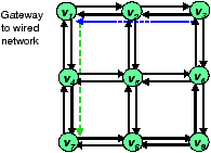
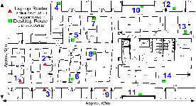
The CRP protocol was deployed on two testbeds: (1) A 14 node wireless testbed running Windows XP (network A), and (2) A 20 node wireless testbed running Mandrake Linux (network B). Network A is located on a floor of an office building in Redmond and is illustrated in Figure 9. 10 of the nodes are small form factor HP desktops each with 3 DLink AWG132 802.11a/b/g USB cards while 4 nodes are Toshiba tablet PCs with one Netgear WAG511 802.11a/b/g PCMCIA card and 2 DLink AWG132 802.11a/b/g cards. The driver configurations are modified to allow multiple cards from the same vendor to co-exist in a machine. The radios on each node have their own SSID and are statically assigned the 802.11a frequencies 5180, 5240 and 5300 GHz. Thus, the 42 radios form three 14-node networks each with its own frequency and SSID glued together through the CRP virtual adapter. Each radio works in ad-hoc mode and performs autorate selection. The OS on each machine implements TCP-SACK. Finally, the nodes are static and use statically assigned private IPv4 addresses. The results are expected to not be significantly affected by external interference since no other 802.11a network was in the area. Network B is located across 3 academic building at Purdue University and is shown in Figure 10. The machines are small form factor HP desktops each with an Atheros 802.11a/b/g radio and run Linux.
We first demonstrate the performance of CRP in a controlled and configurable simulator setting.
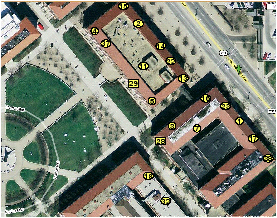
The first scenario demonstrates how CRP can exploit frequency reuse opportunities in a correct way. We consider a chain of 10 nodes separated by 300m, each with 3 radios on 3 orthogonal channels. The transmission power used causes interference to nodes even two hops away which is typical in real networks. Figure 11 shows the routes selected by using WCETT (on top) and CRP (below).
Notice the route selected by WCETT: while it maximizes channel diversity, i.e., each channel is used exactly equally (3 times), it cannot optimize the ordering of the channel use (as explained in Section 2.2) while CRP chooses the optimal route. How does this route selection impact performance? Figure 11 also shows the UDP and TCP throughput achieved using ETT, WCETT and CRP on this chain topology. The results show that CRP route selection has a significant impact on performance improving UDP throughput by 166% over WCETT and over 1000% compared to ETT. For TCP, CRP improves the throughput by around 44% and 91% with respect to WCETT and ETT, respectively. Thus, CRP is able to select a path with high raw capacity. However, the gains are reduced due to TCP's known inability to reach the available bandwidth effectively in multi-hop wireless networks (which is also amplified by the long chain). An interesting aspect to note here is that the benefit comes from using the SIM metric and either CPP or Dijkstra's algorithm would choose the correct route. However, the next section shows when SIM by itself is not enough and demonstrates the usefulness of context-based path selection.
In this scenario, we consider a simple 3 node topology as shown in Figure 12. Node A and B have 2 radios tuned to channel 1 and 2 while node C has one radio tuned to channel 1. Even in such a simple topology, WCETT and ETT are unable to choose the good route which can simply be decided by observation. This is because of the `forgetfulness' of Dijkstra. Once the route to B is decided simply based on the lowest metric to get to B, it cannot be changed. Thus, both ETT and WCETT in MR-LQSR choose the path with both hops on channel 1 while CRP chooses the path with channels 1 and 2 since CRP does not finalize the interface used to reach B right away.
Figure 12 shows that the CRP route improves the TCP throughput by 108% and UDP throughput by 102% over both WCETT and ETT. Note that the performance improvement is similar for TCP and UDP since in a two-hop scenario, TCP is better able to utilize the available bandwidth.
We now evaluate CRP in a large network of 50 static nodes randomly placed in a 2000 m x 2000 m area. We selected 20 random non-overlapping source destination pairs in the network and initiated a TCP connection between each pair for 60 seconds (so as to observe steady state behavior). Each node had 3 radios on orthogonal channels.
The results in Figure 13 shows the percentage increase in TCP throughput of CRP over WCETT. We find that 7 paths have 20% or more gain in TCP throughput with the gains being as high as 90% in some cases. Typically whenever the performance of CRP and WCETT are equal, it is for two reasons: (1) The path is 3 hops or shorter in length. Since WCETT assigns channels in equal proportions, it always chooses a route similar to CRP (each link has a different channel), (2) Although rare, sometimes when the path is longer than 3 hops, by random chance the WCETT ordering of channels turns out to be optimal.
We now evaluate CRP for a single-radio network with network coding in QualNet. Consider the network shown in Figure 2 with an existing flow v3 ⇝ v1. After 3 seconds, v1 initiates a flow to v9. There are many possible routes that this flow can take, but only one (v1−v2−v3−v6−v9) is optimal in terms of the resource consumption. CRP causes the flow v1⇝ v9 to choose the mutually beneficial route v1−v2−v3−v6−v9, resulting in maximized mixing. Intuitively, the existing flow v3⇝ v1 creates a discount in terms of the conditional ERC metric in the opposite direction, which attracts v1 to choose route v1−v2−v3−v6−v9. Once the flows start in both directions, they stay together and mix because both see discounts. As shown in Table 1, CRP increases the number of mixed packets in this scenario by 12× in comparison to LQSR+COPE.
Scenario Mixed (CRP+COPE) Mixed (LQSR+COPE) S1 20,366 1,593 S2 39,576 24,197
Table 1: Gain from CRP+COPE compared to LQSR+COPE.
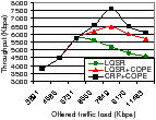
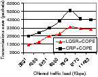
We continue with the 9-node grid network scenario and evaluate the performance with three flows: (1)v9⇝ v1, (2) v1⇝ v9, and (3) v3⇝ v1. Each flow begins randomly between 50–60 seconds into the simulation. We evaluate the performance of LQSR, LQSR+COPE and CRP+COPE for this scenario for different input loads. The results are depicted in Figure 14. CRP provides throughput gains compared to LQSR (up to 47%) and LQSR+COPE (up to 15%). Without CRP, flows mix essentially by chance. In the example, the flow 1-2-3-6-9 is mixed with 9-6-3-2-1 with CRP, due to the mutually beneficial discounts enjoyed by both flows.
Figure 14 also gives the amount of resource saved by using CRP. CRP consistently provides reduction of packet transmissions of over 10,000 packets across a wide variety of traffic demands. Another observation from Figure 14 is that the saved transmissions reduce as the network load increases. This is counter-intuitive since more packets should indicate more mixing opportunities. However, this occurs because of the capture effect in the 802.11 MAC layer which is amplified at high loads. Due to this, packets from only one node (the capturing node) fill queues for large durations of time without allowing other traffic. This reduces mixing opportunities at high load. This problem can potentially be addressed through a better MAC layer design that avoids capture.
Thus, the simulation results for multi-radio networks show that gains from CRP are observed in two cases: (1) When frequency reuse is possible, and (2) When there are heterogeneous nodes in the network, i.e. not all nodes have the same number of interfaces. While these scenarios are common and important to address (typical wireless networks are bound to have some frequency reuse opportunities and networks may have all different types of nodes with different number of radios and characteristics), our testbed evaluation in the next section provides insight into other scenarios where CRP is helpful. In systems with network coding, CRP performance exemplifies that network coding itself cannot provide the best achievable performance and a protocol such as CRP can help network coding achieve better performance.
We now document our experience with the performance of CRP in a real wireless network deployment. We first perform a series of microbenchmarks to see its performance in known settings and then evaluate its performance as a running system.
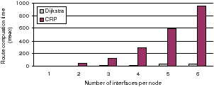
CRP improves Dijkstra route selection at the expense of more computation and complexity. While the complexity is not a hurdle (the protocol is already implemented), it is important to find the computational complexity to ascertain the protocols applicability to real mesh networks which may have embedded devices with slow processors.
We configured our CRP implementation's graph cache with a graph topology of 100 nodes (taken from a typical neighborhood layout) and varied the number of interfaces per node. We then evaluated the time taken by CRP versus Dijkstra in computing the shortest paths to all nodes in the network. We find that our implementation, while significantly more computationally expensive than Dijkstra, can find routes in the extreme case of 100 node networks with 6 radios each in 900 ms. The current MCL implementation in fact calls Dijkstra's algorithm only once per second, caching routes in between. However in our current testbed with 14 nodes each with 42 radios, the computation is performed in around 10-20 ms. Thus, even if we use embedded mesh routers whose CPU speeds are 5-6 times slower than our testbed nodes, we expect to typically find routes under 100 ms. Additionally, one could proactively find such routes in the background to hide this delay as well.
We now evaluate the real performance gains from good choice of routes in our testbed. Note that unlike the simulator which does not simulate adj-channel interference5, this gives us a better idea of the potential performance benefits.
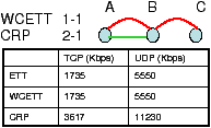
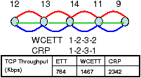
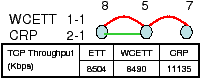
We selected one of the 4 hops routes in testbed A between nodes 12 and 9 and performed multiple 1-minute TCP transfers taking the median performance. The route and channels chosen by WCETT and CRP are shown in Figure 16. WCETT reuses channel 2 on the last link 11→9 essentially because the channel 2 radio on node 11 had a lower ETT. Thus, WCETT took a local view not realizing this link would cause secondary interference with link 13→14. However, CRP chose the interface on channel 1 on the last link which although locally had a higher ETT, did not cause self-interference. Thus this route got a higher SIM score and was selected by CRP providing a performance gain of 60% and close to 200% with respect to WCETT and ETT respectively. This example clearly shows how using context benefit translates into real world gain.
We next consider the simple topology of 3 to see how much gain a CRP provides over a WCETT route in the real world. As shown in Figure 17, we configured node 8 and 5 with two interfaces on channel 1 and 2 while node 7 had one interface on channel 1.
WCETT chose channel 1 on both links due to the the use of Dijkstra and ETT also chose this route because the ETT of channel 2 on node 8 was around 1ms higher than channel 1. However, CRP is able to identify the correct route and chooses a route with channel 2 and channel 1. This allows CRP to have a TCP throughput 31% higher than both WCETT and ETT. Note that the gain is lower than that observed in simulation because some adj-channel interference can limit gains. From measurements, we know such interference exists despite our attempts to place the cards at some distance from each other on each machine.
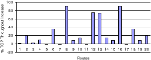
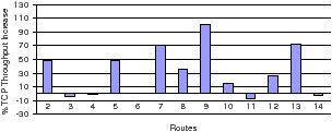
We now evaluate the gain from CRP in a running network topology. Each testbed node in this scenario has 3 radios. We performed multiple 1-minute TCP transfers between node 1 and all the other testbed nodes with WCETT and CRP. The % throughput gain of CRP over WCETT observed from node 1 to the other nodes (numbered on the x-axis) is shown in Figures 18.
The results show that CRP can improve WCETT throughput in 7 out of 13 paths by up to 100% and more than 30% on most paths. Some of the results are expected while some are non-intuitive. Among the expected results are: (1) The paths to nodes 3, 6, 4 and 116 have no gain since they are less than 4 hops in length and WCETT can assign costs correctly if the number of hops are less than the number of radios per node. (2) Nodes 5 and 7 are reached via 4-hop routes and the SIM metric can now choose a better path to provide gain.
Among the unexpected results are: (1) Paths to nodes 8 and 9 have gain despite their being 3 hops away. We found this was caused by ETT variation among the interfaces of node 6 which rendered 2 interfaces almost useless due to high ETTs and effectively caused a bottleneck link which required careful route selection. CRP identified and used the good interface on node 6 and thus performed better. (2) Routes to node 10 have low gain despite reuse opportunities since the link performance is constrained by the weak link 8→10. However, going to nodes 12 and 13 through 10 gives gain since the throughput is now constrained more by ordering of channels selected than the weak link. (3) Finally, although 14 is 4 hops away, there is no gain because WCETT chooses the good route selected by CRP purely by chance.
We also evaluated the gain in a heterogeneous network scenario where all nodes do not have the same number of interfaces. In these experiments, gains of up to 152% were observed.
We now perform experiments with our Linux CRP implementation on top of COPE in testbed B. We take multiple examples of the Alice-and-Bob topologies from our testbed and demonstrate how much gain is provided by simply using SrcRR+COPE versus using CRP+COPE. This testbed has only one radio on each node. We use the ERC metric in CRP. Table 2 shows the gains achieved using CRP for different topologies tested in the testbed. The left hand column lists the two flows initiated in the network in each case and the node numbers refer to Figure 10.
Scenarios UDP Gain TCP Gain 22→3, 3→22 1.66× 1.29× 18→5, 5→18 1.53× 1.24× 11→7, 7→11 1.78× 1.31× 37→13, 2→5 1.71× 1.24×
Table 2: Median throughput gain from CRP+COPE compared to LQSR+COPE for both UDP and TCP. For each scenario we initiated the flows 15 times.
The table shows significant gains from CRP+COPE over SrcRR+COPE in the range of 1.7× for UDP and 1.27× for TCP. In the first scenario, SrcRR chooses the routes 22-13-3 and 3-5-22 which does not provide gain from network coding while causing interference among the two flows. CRP entices flow 3-22 onto the same route due to the ERC discounts and allows network coding to occur at node 13 for the duration of the transfer. In the second scenario under SrcRR, flow 18-5 uses the route 18-28-5 while flow 5-18 uses the low quality direct route 5-18. CRP advertises discounts on the 28-18 link for traffic from 5 and this causes the two flows to mix at node 28 resulting in gain. In the third scenario, SrcRR choose the routes 11-5-3-7 and 7-16-13-11/7-16-5-11 for the two flows resulting in no coding of packets while CRP brings the two flows onto a mutually beneficial route traversing nodes 5 and 3 in both directions. Finally in the fourth scenario, CRP allows nodes 37 and 2 to choose 11 as a next hop once ERC discounts become visible. Node 5 and 13 can overhear the packets from 37 and 2 respectively giving rise to network coding gain. Without CRP the two flows tend to take the routes 37-11-5 and 2-14-22 resulting in no coding gain. Thus, we can see the benefits that CRP provides to the COPE system allows the network coding engine more opportunities to code packets. Note that if a lot of flows are present in the network (such as the scenarios evaluated in [6]), the benefits from CRP would be less significant since a large number of packets present in the network can provide enough coding opportunities without intelligent route selection. However, CRP can provide COPE with coding opportunities even in more sparse or lightly loaded networks.
Note that we currently do not aim at solving the load balanced routing problem in handling multiple flows. We believe a better practical strategy is for link traffic to affect the link metric and then use a method, such as CRP, to find a route. Thus CRP should potentially be useful for load-balanced routing proposals.
In this paper, we investigated context-based routing, a general route selection framework that models link interdependencies and selects good routes, through the case studies of network coding–aware routing and self-interference aware routing in multi-radio systems. The effectiveness of our approach is demonstrated through both simulations and a deployed implementation. In the future, we plan to investigate other potential applications for CRP by studying further scenarios where link interdependencies exists such as multi-radio networks with network coding or lightpath selection in WDM optical networks.
This work was supported in part by NSF grant CNS-0626703. We thank the reviewers and our shepherd Sue Moon for their comments.
This document was translated from LATEX by HEVEA.