Load Shedding in Network Monitoring
Applications
Pere Barlet-Ros*, Gianluca Iannaccone+, Josep Sanjuŕs-Cuxart*,
Diego Amores-López*, Josep Solé-Pareta*
* Technical University of Catalonia (UPC), Barcelona, Spain
+ Intel Research, Berkeley, CA
Abstract
Monitoring and mining real-time network data streams is crucial for managing and
operating data networks. The information that network operators desire to extract
from the network traffic is of different size, granularity and accuracy depending on
the measurement task (e.g., relevant data for capacity planning and intrusion
detection are very different). To satisfy these different demands, a new class of
monitoring systems is emerging to handle multiple arbitrary and continuous
traffic queries. Such systems must cope with the effects of overload situations
due to the large volumes, high data rates and bursty nature of the network
traffic.
In this paper, we present the design and evaluation of a system that
can shed excess load in the presence of extreme traffic conditions, while
maintaining the accuracy of the traffic queries within acceptable levels. The
main novelty of our approach is that it is able to operate without explicit
knowledge of the traffic queries. Instead, it extracts a set of features from the
traffic streams to build an on-line prediction model of the query resource
requirements. This way the monitoring system preserves a high degree of flexibility,
increasing the range of applications and network scenarios where it can be
used.
We implemented our scheme in an existing network monitoring system and
deployed it in a research ISP network. Our results show that the system
predicts the resources required to run each traffic query with errors below
5%, and that it can efficiently handle extreme load situations, preventing
uncontrolled packet losses, with minimum impact on the accuracy of the queries’
results.
1 Introduction
Network monitoring applications that must extract a large number of real-time
metrics from many input streams are becoming increasingly common. These include
for example applications that correlate network data from multiple sources (e.g.,
end-systems, access points, switches) to identify anomalous behaviors, enable traffic
engineering and capacity planning or manage and troubleshoot the network
infrastructure.
The main challenge in these systems is to keep up with ever increasing input data
rates and processing requirements. Data rates are driven by the increase in network
link speeds, application demands and the number of end-hosts in the network. The
processing requirements are growing to satisfy the demands for fine grained and
continuous analysis, tracking and inspection of network traffic. This challenge is
made even harder as network operators expect the queries to return accurate
enough results in the presence of extreme or anomalous traffic patterns,
when the system is under additional stress (and the query results are most
valuable!). The alternative of over-provisioning the system to handle peak rates or
any possible traffic mix would be prohibitively expensive and result in a
highly underutilized system based on an extremely pessimistic estimation of
workload.
Recently, several research proposals have addressed this challenge [18, 22, 23, 8, 14].
The solutions introduced belong to two broad categories. The first includes
approaches that consider a pre-defined set of metrics and can report approximate
results (within given accuracy bounds) in the case of overload [18, 14]. The second
category includes solutions that define a declarative query language with a small set
of operators for which the resource usage is assumed to be known [22, 23, 8]. In the
presence of overload, operator-specific load shedding techniques are implemented
(e.g., selectively discarding some records, computing approximate summaries) so
that the accuracy of the entire query is preserved within certain bounds.
These solutions present two common limitations: (i) they restrict the types of
metrics that can be extracted from the traffic streams, limiting therefore
the possible uses and applications of these systems, and (ii) they assume
explicit knowledge of the cost and selectivity of each operator, requiring a very
careful and time-consuming design and implementation phase for each of
them.
In this paper, we present a system that supports multiple arbitrary and
continuous traffic queries on the input streams. The system can handle overload
situations due to anomalous or extreme traffic mixes by gracefully degrading the
accuracy of the queries. The core of our load shedding scheme consists of the
real-time modeling and prediction of the system resource usage that allows the
system to anticipate future bursts in the resource requirements. The main novelty of
our approach is that it does not require explicit knowledge of the query or of the
types of computations it performs (e.g., flow classification, maintaining aggregate
counters, string search). This way we preserve the flexibility of the monitoring
system, enabling fast implementation and deployment of new network monitoring
applications.
Without any knowledge of the computations performed on the packet streams, we
infer their cost from the relation between a large set of pre-defined “features” of the
input stream and the actual resource usage. A feature is a counter that describes a
specific property of a sequence of packets (e.g., number of unique source IP
addresses). The features we compute on the input stream have the advantage of
being lightweight with a deterministic worst case computational cost. Then, we
automatically identify those features that best model the resource usage of each
query and use them to predict the overall load of the system. This short-term
prediction is used to guide the system on deciding when, where and how much load to
shed. In the presence of overload, the system can apply several load shedding
techniques, such as packet sampling, flow sampling or computing summaries of the
data streams to reduce the amount of resources required by the queries to
run.
For simplicity, in this paper we focus only on one resource: the CPU cycles. Other
system resources are also critical (e.g., memory, disk bandwidth and disk space) and
we believe that approaches similar to what we propose here could be applied as
well.
We have integrated our load shedding scheme into the CoMo monitoring
system [16] and deployed it on a research ISP network, where the traffic load
and query requirements exceed by far the system capacity. We ran a set of
seven concurrent queries that range from maintaining simple counters (e.g.,
number of packets, application breakdown) to more complex data structures
(e.g., per-flow classification, ranking of most popular destinations or pattern
search).
Our results show that, with the load shedding mechanism in place, the system
effectively handles extreme load situations, while being always responsive and
preventing uncontrolled packet losses. The results also indicate that a predictive
approach can quickly adapt to overload situations and keep the queries’ results
within acceptable error bounds, as compared to a reactive load shedding
strategy.
The remainder of this paper is structured as follows. Section 2 presents in greater
detail some related work. Section 3 introduces the monitoring system and the set of
queries we use for our study. We describe our prediction method in Section 4
and validate its performance using real-world packet traces in Section 5.
Section 6 presents a load shedding scheme based on our prediction method.
Finally, in Section 7 we evaluate our load shedding scheme in a research ISP
network, while Section 8 concludes the paper and introduces ideas for future
work.
2 Related Work
The design of mechanisms to handle overload situations is a classical problem in any
real-time system design and several previous works have proposed solutions in
different environments.
In the network monitoring space, NetFlow [9] is considered the state-of-the-art.
In order to handle the large volumes of data exported and to reduce the load on the
router it resorts to packet sampling. The sampling rate must be defined
at configuration time and network operators tend to set it to a low “safe”
value (e.g., 1/100 or 1/1000 packets) to handle unexpected traffic scenarios.
Adaptive NetFlow [14] allows routers to dynamically tune the sampling
rate to the memory consumption in order to maximize the accuracy given
a specific incoming traffic mix. Keys et al. [18] extend the approach used
in NetFlow by extracting and exporting a set of 12 traffic summaries that
allow the system to answer a fixed number of common questions asked by
network operators. They deal with extreme traffic conditions using adaptive
sampling and memory-efficient counting algorithms. Our work differs from these
approaches in that we are not limited to a fixed set of known traffic reports, but
instead we can handle arbitrary network traffic queries, increasing the range of
applications and network scenarios where the monitoring system can be
used.
Several research proposals in the stream database literature are also very
relevant to our work. The Aurora system [5] can process a large number of
concurrent queries that are built out of a small set of operators. In Aurora, load
shedding is achieved by inserting additional drop operators in the data flow
of each query [23]. In order to find the proper location to insert the drop
operators, [23] assumes explicit knowledge of the cost and selectivity of each
operator in the data flow. In [7, 22], the authors propose a system that applies
approximate query processing techniques, instead of dropping records, to
provide approximate and delay-bounded answers in presence of overload. On
the contrary, in our context we have no explicit knowledge of the query
and therefore we cannot make any assumption on its cost or selectivity to
know when it is the right time to drop records. Regarding the records to
be dropped, we apply packet or flow sampling to reduce the load on the
system, but other summarization techniques are an important piece of future
work.
In the Internet services space, SEDA [24] proposes an architecture to develop
highly concurrent server applications, built as networks of stages interconnected by
queues. SEDA implements a reactive load shedding scheme by dropping incoming
requests when an overload situation is detected (e.g., the response time of the system
exceeds a given threshold). In this work we use instead a predictive approach to
anticipate overload situations. We will show later how a predictive approach
can significantly reduce the impact of overload as compared to a reactive
one.
Finally, our system is based on extracting features from the traffic streams with
deterministic worst case time bounds. Several solutions have been proposed in
the literature to this end. For example, counting the number of distinct
items in a stream has been addressed in the past in [15, 1]. In this work we
implement the multi-resolution bitmap algorithms for counting flows proposed
in [15].
3 System Overview
The basic thesis behind this work is that the cost of maintaining the data
structures needed to execute a query can be modeled by looking at a set of traffic
features that characterizes the input data. The intuition behind this thesis
comes from the empirical observation that each query incurs a different
overhead when performing basic operations on the state it maintains while
processing the input packet stream (e.g., creating new entries, updating
existing ones or looking for a valid match). We observed that the time spent by
a query is mostly dominated by the overhead of some of these operations
and therefore can be modeled by considering the right set of simple traffic
features.
A traffic feature is a counter that describes a property of a sequence of packets.
For example, potential features could be the number of packets or bytes in the
sequence, the number of unique source IP addresses, etc. In this paper we will select
a large set of simple features that have the same underlying property: deterministic
worst case computational complexity.
Once a large number of features is efficiently extracted from the traffic
stream, the challenge is in identifying the right ones that can be used to
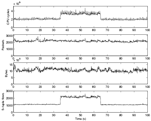
accurately model and predict the query’s CPU usage. Figure 1 illustrates a
very simple example. The figure shows the time series of the CPU cycles
consumed by an “unknown” query (top graph) when running over a 100s
snapshot of our dataset (described in Section 5.1), where we inserted an
artificially generated anomaly. The three bottom plots show three possible
features over time: the number of packets, bytes and flows (defined by the
classical 5-tuple: source and destination addresses, source and destination
port numbers and protocol number). It is clear from the figure that the
bottom plot would give us more useful information to predict the CPU usage
over time for this query. It is also easy to infer that the query is performing
some sort of per-flow classification, hence the higher cost when the number
of flows increases, despite the volume of packets and bytes remains fairly
stable.
We designed a method that automatically selects the most relevant feature(s)
from small sequences of packets and uses them to accurately predict the CPU
usage of arbitrary queries. This fine-grained and short-term prediction is
then used to quickly adapt to overload situations by sampling the input
streams.
3.1 Monitoring Platform
We chose the CoMo platform [16] to develop and evaluate our resource usage
prediction and load shedding methods. CoMo is an open-source passive monitoring
system that allows for fast implementation and deployment of network monitoring
applications. CoMo follows a modular approach where users can easily define traffic
queries as plug-in modules written in C, making use of a feature-rich API
provided by the core platform. Users are also required to specify a simple
stateless filter to be applied on the incoming packet stream (it could be
all the packets) as well as the granularity of the measurements, hereafter
called measurement interval (i.e., the time interval that will be used to report
continuous query results). All complex stateful computations are contained
within the plug-in module code. This approach allows users to define traffic
queries that otherwise could not be easily expressed using common declarative
languages (e.g., SQL). More details about the CoMo platform can be found
in [16].
In order to provide the user with maximum flexibility when writing queries,
CoMo does not restrict the type of computations that a plug-in module
can perform. As a consequence, the platform does not have any explicit
knowledge of the data structures used by the plug-in modules or the cost of
maintaining them. Therefore, any load shedding mechanism for such a system must
operate only with external observations of the CPU requirements of the
modules – and these are not known in advance but only after a packet has been
processed.
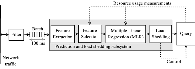
Figure 2 shows the components and the data flow in the system. The prediction
and load shedding subsystem (in gray) intercepts the packets from the filter before
they are sent to the plug-in module implementing the traffic query. The system
operates in four phases. First, it groups each 100ms of traffic in a “batch” of
packets1. Each batch is then processed to extract a large pre-defined set of
traffic features (Section 4.1). The feature selection subsystem is in charge of
selecting the most relevant features according to the recent history of the
query’s CPU usage (Section 4.3). This phase is important to reduce the
cost of the prediction algorithm, because it allows the system to discard
beforehand the features regarded as useless for prediction purposes. This subset of
relevant features is then given as input to the multiple linear regression
subsystem to predict the CPU cycles required by the query to process the entire
batch (Section 4.2). If the prediction exceeds the system capacity, the load
shedding subsystem pre-processes the batch to discard (via packet or flow
sampling) a portion of the packets (Section 6). Finally, the actual CPU usage
is computed and fed back to the prediction subsystem to close the loop
(Section 4.4).
3.2 Queries
Despite the fact that the actual metric computed by the query is not relevant for our
work – our system considers all queries as black boxes – we are interested in
considering a wide range of queries when performing the evaluation. We have selected
the set of queries that are part of the standard distribution of CoMo2. Table 1
provides a brief summary of the queries. We believe that these queries form a
representative set of typical uses of a real-time network monitoring system. They
present different CPU usage profiles for the same input traffic and use different data
structures to maintain their state (e.g., aggregated counters, arrays, hash tables,
linked lists).
|
| | Name | Description |
|
| | application | Port-based application classification |
|
| | flows | Per-flow counters |
|
| | high-watermark | High watermark of link utilization |
|
| | link-count | Traffic load |
|
| | pattern search | Identifies sequences of bytes in the payload |
|
| | top destinations | Per-flow counters for the top-10 destination IPs |
|
| | trace | Full-payload collection |
|
| | |
| Table 1: | Queries used in the experimental evaluation |
|
4 Prediction Methodology
In this section we describe in detail the three phases that our system executes to
perform the prediction (i.e., feature extraction, feature selection and multiple linear
regression) and how the resource usage is monitored. The only information
we require from the continuous query is the measurement interval of the
results. Avoiding the use of additional information increases the range of
applications where this approach can be used and also reduces the likelihood
of compromising the system by providing incorrect information about a
query.
4.1 Feature Extraction
We are interested in finding a set of traffic features that are simple and inexpensive
to compute, while helpful to characterize the CPU usage of a wide range of queries. A
feature that is too specific may allow us to predict a given query with great
accuracy, but could have a cost comparable to directly answering the query
(e.g., counting the packets that contain a given pattern to predict the cost
of signature-based IDS-like queries). Our goal is therefore to find features
that may not explain in detail the entire cost of a query, but can provide
enough information about the aspects that dominate the processing cost.
For instance, in the previous example of a signature-based IDS query, the
cost of matching a string will mainly depend on the number of collected
bytes.
In addition to the number of packets and bytes, we maintain four counters per
traffic aggregate that are updated every time a batch is received. A traffic aggregate
considers one or more of the TCP/IP header fields: source and destination IP
addresses, source and destination port numbers and protocol number. The four
counters we monitor per aggregate are: (i) the number of unique items in
the batch; (ii) the number of new items compared to all items seen in a
measurement interval; (iii) the number of repeated items in the batch (i.e.,
items in the batch minus unique) and (iv) the number of repeated items
compared to all items in a measurement interval (i.e., items in the batch minus
new).
For example, we may aggregate packets based on the source IP address and
source port number, and then count the number of unique, new and repeated
source IP address and source port pairs. Table 2 shows the combinations of
the five header fields considered in this work. Although we do not evaluate
other choices here, we note that other aggregates may also be useful (e.g.,
source IP prefixes or other combinations of the 5 header fields). Adding
new traffic features (e.g., payload-related features) as well as considering
other combinations of the existing ones is an important part of our future
work.
|
| | No. | Traffic aggregate |
|
| | 1 | src-ip |
|
| | 2 | dst-ip |
|
| | 3 | protocol |
|
| | 4 | <src-ip, dst-ip> |
|
| | 5 | <src-port, proto> |
|
| | 6 | <dst-port, proto> |
|
| | 7 | <src-ip, src-port, proto> |
|
| | 8 | <dst-ip, dst-port, proto> |
|
| | 9 | <src-port, dst-port, proto> |
|
| | 10 | <src-ip, dst-ip, src-port, dst-port, proto> |
|
| | |
| Table 2: | Set of traffic aggregates (built from combinations of TCP/IP header
fields) used by the prediction |
|
This large set of features (four counters per traffic aggregate plus the total packet
and byte counts, i.e., 42 in our experiments) helps narrow down which basic
operations performed by the queries dominate their processing costs (e.g.,
creating a new entry, updating an existing one or looking up entries). For
example, the new items are relevant to predict the CPU requirements of
those queries that spend most time creating entries in the data structures,
while the repeated items feature may be relevant to queries where the cost
of updating the data structures is much higher than the cost of creating
entries.
In order to extract the features with minimum overhead, we implement the
multi-resolution bitmap algorithms proposed in [15]. The advantage of the
multi-resolution bitmaps is that they bound the number of memory accesses per
packet as compared to classical hash tables and they can handle a large
number of items with good accuracy and smaller memory footprint than
linear counting [25] or bloom filters [4]. We dimension the multi-resolution
bitmaps to obtain counting errors around 1% given the link speeds in our
testbed.
4.2 Multiple Linear Regression
Regression analysis is a widely applied technique to study the relationship between a
response variable  and one or more predictor variables
  . The
linear regression model assumes that the response variable
. The
linear regression model assumes that the response variable  is a linear function of
the
is a linear function of
the 
 predictor variables3. The fact that this relationship exists can be
exploited for predicting the expected value of
predictor variables3. The fact that this relationship exists can be
exploited for predicting the expected value of  (i.e., the CPU usage) when
the values of the
(i.e., the CPU usage) when
the values of the  predictor variables (i.e., the individual features) are
known.
predictor variables (i.e., the individual features) are
known.
When only one predictor variable is used, the regression model is often referred to
as simple linear regression (SLR). Using just one predictor has two major drawbacks.
First, there is no single predictor that yields good performance for all queries. For
example, the CPU usage of the link-count query can be well modeled by
looking at the number of packets in the batch, while the trace query would be
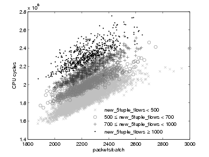
better modeled by the number of bytes. Second, the CPU usage of more
complex queries may depend on more than a single feature. To illustrate
this latter point, we plot in Figure 3 the CPU usage for the flows query
versus the number of packets in the batch. As we can observe, there are
several underlying trends that depend both on the number of packets and
on the number of new 5-tuples in the batch. This behavior is due to the
particular implementation of the flows query that maintains a hash table to
keep track of the flows and expires them at the end of each measurement
interval.
Multiple linear regression (MLR) extends the simple linear regression model to
several predictor variables. The general form of a linear regression model for p
predictor variables can be written as follows [10]:
 | (1) |
In fact, Equation 1 corresponds to a system of equations that in matrix notation can
be written as:
 | (2) |
where Y is a n× 1 column vector of the response variable observations (i.e., the CPU
usage of the previous n batches processed by the query); X is a n × (p + 1) matrix
resulting from n observations of the p predictor variables X1,…,Xp (i.e., the values of
the p features extracted from the previous n batches) with a first column of 1’s
that represents the intercept term β0; β is a (p + 1) × 1 column vector of
unknown parameters  (
( are referred to as the
regression coefficients or weights); and ɛ is a n × 1 column vector of n residuals
ɛi.
are referred to as the
regression coefficients or weights); and ɛ is a n × 1 column vector of n residuals
ɛi.
The estimators b of the regression coefficients β are obtained by the Ordinary
Least Squares (OLS) procedure, which consists of choosing the values of
the unknown parameters b0,…,bp in such a way that the sum of squares
of the residuals is minimized. In our implementation, we use the singular
value decomposition (SVD) method [21] to compute the OLS. Although
SVD is more expensive than other methods, it is able to obtain the best
approximation, in the least-squares sense, in the case of an over- or underdetermined
system.
The statistical properties of the OLS estimators lie on some assumptions that
must be fulfilled [10, pp. 216]: (i) the rank of X is p + 1 and is less than n, i.e., there
are no exact linear relationships among the X variables (no multicollinearity); (ii) the
variable ɛi is normally distributed and the expected value of the vector ɛ is zero; (iii)
there is no correlation between the residuals and they exhibit constant variance; (iv)
the covariance between the predictors and the residuals is zero. In Section 4.3 we
present a technique that makes sure the first assumption is valid. We have also
verified experimentally using the packet traces of our dataset that the other
assumptions hold but in the interest of space we will not show the results
here.
4.3 Feature Selection
Since we assume arbitrary queries, we cannot know in advance which features should
be used as predictors in the MLR for each query. Including all the extracted traffic
features in the regression has several drawbacks: (i) the cost of the linear regression
increases quadratically with the number of predictors, much faster than the gain in
terms of accuracy (irrelevant predictors); (ii) even including all possible
predictors, there would still be a certain amount of randomness that cannot
be explained by any predictor; (iii) predictors that are linear functions of
other predictors (redundant predictors) invalidate the no multicollinearity
assumption4.
It is therefore important to identify a small subset of features to be used as
predictors. In order to support arbitrary queries, we need to define a generic
feature selection algorithm. We would also like our method to be capable
of dynamically selecting different sets of features if the traffic conditions
change during the execution, and the current prediction model becomes
obsolete.
Most of the algorithms proposed in the literature are based on a sequential
variable selection procedure [10]. However, they are usually too expensive to be used
in a real-time system. For this reason, we decided to use a variant of the Fast
Correlation-Based Filter (FCBF) [26], which can effectively remove both irrelevant
and redundant features and is computationally very efficient. Our variant differs from
the original FCBF algorithm in that we use the linear correlation coefficient as a
predictor goodness measure, instead of the symmetrical uncertainty measure used
in [26].
The algorithm consists of two main phases. First, the linear correlation coefficient
between each predictor and the response variable is computed and the predictors
with a coefficient below a pre-defined FCBF threshold are discarded as not
relevant. In Section 5.2 we will address the problem of choosing the appropriate
FCBF threshold. Second, the predictors that are left after the first phase
are ranked according to their coefficient values and processed iteratively to
discard redundant predictors (i.e., predictors that have a mutual strong
correlation), as described in [3]. The overall complexity of the FCBF is
O(n p log p), where n is the number of observations and p the number of
predictors [26].
4.4 Measurement of System Resources
Fine grained measurement of CPU usage is not an easy task. The mechanisms
provided by the operating system do not offer enough resolution for our purposes,
while processor performance profiling tools [17] impose a large overhead and are not
a viable permanent solution.
In this work, we use instead the time-stamp counter (TSC) to measure the CPU
usage, which is a 64-bit counter incremented by the processor every clock cycle [17].
In particular, we read the TSC before and after a batch is processed by a query. The
difference between these two values corresponds to the number of CPU cycles used by
the query to process the batch.
The CPU usage measurements that are fed back to the prediction system should
be accurate and free of external noise to reduce the errors in the prediction. However,
we empirically detected that measuring CPU usage at very small timescales incurs in
several sources of noise:
Instruction reordering. The processor can reorder instructions at run time in
order to improve performance. In practice, the rdtsc instruction used to read the
TSC counter is often reordered, since it simply consists of reading a register and it
has no dependencies with other instructions. To avoid the effects of reordering, we
execute a serializing instruction (e.g., cpuid) before and after our measurements [17].
Since the use of serializing instructions can have a severe impact on the
system performance, we only take two TSC readings per query and batch,
and we do not take any partial measurements during the execution of the
query.
Context switches. The operating system may decide to schedule out the query
process between two consecutive readings of the TSC. In that case, we would be
measuring not only cycles belonging to the query, but also cycles of the process (or
processes) that are preempting the query.
In order to avoid degrading the accuracy of future predictions when a context
switch happens during a measurement, we discard those observations from the
history and replace them with our prediction. To measure context switches, we
monitor the rusage process structure in the Linux kernel.
Disk accesses. Disk accesses can interfere with the CPU cycles needed to process a
query. In CoMo, a separate process is responsible for scheduling disk accesses to read
and write query results. In practice, since disk transfers are done asynchronously by
DMA, memory accesses of queries have to compete for the system bus with disk
transfers. For the interested reader we show the limited impact of disk accesses on
the prediction accuracy in [3].
It is important to note that all the sources of noise we detected so far are
independent from the input traffic. Therefore, they cannot be exploited by a
malicious user trying to introduce errors in our CPU measurements to attack the
monitoring system.
5 Validation
In this section we show the performance of our prediction method on real-world
traffic traces. In order to understand the impact of each parameter, we study the
prediction subsystem in isolation from the sources of measurement noise identified in
Section 4.4. We disabled the disk accesses in the CoMo process responsible for
storage operations to avoid competition for the system bus. In Section 7, we will
evaluate our method in a fully operational system.
To measure the performance of our method we consider the relative error in the
CPU usage prediction while executing the seven queries defined in Table 1 over the
traces in our dataset. The relative error is defined as the absolute value of one minus
the ratio of the prediction and the actual number of CPU cycles spent by the
queries over each batch. A more detailed performance analysis can be found
in [3].
5.1 Dataset
We collected two 30-minute traces from one direction of the Gigabit Ethernet link
that connects the Catalan Research and Education Network (Scientific Ring) to
the global Internet via its Spanish counterpart (RedIRIS). The Scientific
Ring is managed by the Supercomputing Center of Catalonia (CESCA) and
connects more than fifty Catalan universities and research centers using many
different technologies that range from ADSL to Gigabit Ethernet [19]. A
trace collected at this capture point is publicly available in the NLANR
repository [20].
The first trace contains only packet headers, while the second one includes
the entire packet payloads instead. Details of the traces are presented in
Table 3.
|
|
|
|
|
Trace name |
Date |
Time | Pkts | Link load (Mbps) |
| | | |
| | | | | (M) | mean/max/min |
|
|
|
|
| | w/o payloads | 02/Nov/05 | 4:30pm-5pm | 103.7 | 360.5/483.3/197.3 |
|
|
|
|
| | with payloads | 11/Apr/06 | 8am-8:30am | 49.4 | 133.0/212.2/096.1 |
|
|
|
|
| | |
| Table 3: | Traces used in the validation |
|
5.2 Prediction Parameters
In our system, two configuration parameters impact the cost and accuracy of the
predictions: the number of observations (i.e., n or the “history” of the system) and
the FCBF threshold used to select the relevant features.
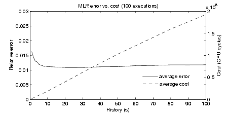
Number of observations. Figure 4 shows the average cost of computing the MLR
versus the prediction accuracy over multiple executions, with values of history
ranging from 1s to 100s (i.e., 10 to 1000 batches). As we can see, the cost grows
linearly with the amount of history, since every additional observation translates
into a new equation in the system in (2). The relative error between the
prediction and the actual number of CPU cycles spent by the queries stabilizes
around 1.2% for histories longer than 6 seconds. Larger errors for very small
amounts of history (e.g., 1s) are due to the fact that the number of predictors
(i.e., p = 42) is larger than the amount of history (i.e., n = 10 batches) and
thus the no multicollinearity assumption is not met. We also checked that
histories longer than 100s do not improve the accuracy, because events that are
not modeled by the traffic features are probably contributing to the error.
Moreover, a longer history makes the prediction model less responsive to
sudden changes in the traffic that may change the behavior of a query. In the
rest of the paper we use a number of observations equal to 60 batches (i.e.,
6s).
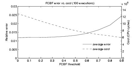
FCBF threshold. The FCBF threshold determines which traffic features are
relevant and not redundant in modeling the response variable. Figure 5 presents the
prediction cost and accuracy as functions of the FCBF threshold over multiple
executions in our testbed, with threshold values ranging from 0 (i.e., all features are
considered relevant but the redundant ones are not selected) to 0.9 (i.e., most
features are not selected). The prediction cost includes both the cost of the selection
algorithm and the cost of computing the MLR with the selected features. Comparing
this graph with Figure 4, we can see that using FCBF reduces the overall cost of the
prediction by more than an order of magnitude while maintaining similar
accuracy.
As the threshold increases, less predictors are selected, and this turns into a
decrease in the CPU cycles needed to run the MLR. However, the error remains fairly
close to the minimum value obtained when all features are selected, and starts to
ramp up only for relatively large values of the threshold (around 0.6). Very large
values of the threshold (above 0.8) experience a much faster increase in the error
compared to the decrease in the cost. In the rest of the paper we use a value of 0.6
for the FCBF threshold that achieves a good trade-off between prediction cost and
accuracy.
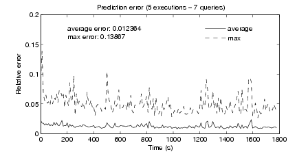
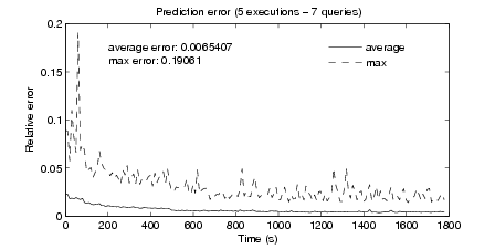
5.3 Prediction Accuracy
In order to evaluate the performance of our method we ran the seven queries of
Table 1 over the two traces in our dataset. Figures 6 and 7 show the time series of
the average and maximum error over five executions when running on the packet
trace with and without payloads, respectively.
The average error in both cases is consistently below 2%, while the maximum
error peaks around 10%. These larger errors are due to external system events
unrelated to the traffic that cause a spike in the CPU usage (e.g., cache misses) or
due to a sudden change in the traffic patterns that is not appropriately modeled by
the features that the prediction is using at that time. However, the time series shows
that our method is able to converge very quickly. The trace without payloads
(Figure 7) exhibits better performance, with average errors that drop well below
1%.
In Table 4, we show the breakdown of the prediction errors by query. The average
error is very low for each query, with a relatively small standard deviation indicating
compact distributions for the prediction errors. As expected, queries that
make use of more complex data structures (e.g., flows, pattern search and
top destinations) incur in the larger errors, but still at most around 3% on
average.
| Trace with payloads
| | Query | Mean | Stdev | Selected features |
|
|
|
| | application | 0.0110 | 0.0095 | packets, bytes |
| flows | 0.0319 | 0.0302 | new dst-ip, dst-port, proto |
| high-watermark | 0.0064 | 0.0077 | packets |
| link-count | 0.0048 | 0.0066 | packets |
| pattern search | 0.0198 | 0.0169 | bytes |
| top destinations | 0.0169 | 0.0267 | packets |
| trace | 0.0090 | 0.0137 | bytes, packets |
| |
| |
|
Trace without payloads
| | Query | Mean | Stdev | Selected features |
|
|
|
| | application | 0.0068 | 0.0060 | repeated 5-tuple, packets |
| flows | 0.0252 | 0.0203 | new dst-ip, dst-port, proto |
| high-watermark | 0.0059 | 0.0063 | packets |
| link-count | 0.0046 | 0.0053 | packets |
| pattern search | 0.0098 | 0.0093 | packets |
| top destinations | 0.0136 | 0.0183 | new 5-tuple, packets |
| trace | 0.0092 | 0.0132 | packets |
| Table 4: | Breakdown of prediction error and selected features by query (5
executions) |
|
It is also very interesting to look at the features that the selection algorithm
identifies as most relevant for each query. Remember that the selection algorithm has
no information about what computations the queries perform nor what type of
packet traces they are processing. The selected features give hints on what a query is
actually doing and how it is implemented. For example, the number of bytes is the
predominant traffic feature for the pattern search and trace queries when running on
the trace with payloads. However, when processing the trace with just packet
headers, the number of packets becomes the most relevant feature for these queries,
as expected.
5.4 Prediction Cost
To understand the cost of running the prediction, we compare the CPU cycles of the
prediction subsystem to those spent by the entire CoMo system over 5 executions.
The feature extraction phase constitutes the bulk of the processing cost, with an
overhead of 9.07%. The overhead introduced by the feature selection algorithm is
only around 1.70% and the MLR imposes an even lower overhead (0.20%), mainly
due to the fact that, when using the FCBF, the number of predictors is significantly
reduced and thus there is a smaller number of variables to estimate. The use of the
FCBF allows to increase the number of features without affecting the cost of
the MLR. Finally, the total overhead imposed by our prediction method is
10.97%
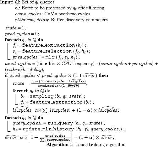
6 Load Shedding
In this section, we provide the answers to the three fundamental questions any
load shedding scheme needs to address: (i) when to shed load (i.e., which
batch), (ii) where to shed load (i.e., which query) and (iii) how much load
to shed (e.g., the sampling rate to apply). Algorithm 1 presents our load
shedding scheme in detail, which controls the Prediction and Load Shedding
subsystem of Figure 2. It is executed at each time bin (i.e., 0.1s in our current
implementation) right after every batch arrival, as described in Section 3.1.
This way, the system can quickly adapt to changes in the traffic patterns by
selecting a different set of features if the current prediction model becomes
obsolete.
6.1 When to Shed Load
To decide when to shed load the system maintains a threshold (avail_cycles) that
accounts for the amount of cycles available in a time bin to process the queries. Since
batch arrivals are periodic, this threshold can be dynamically computed as
(time bin × CPUfrequency) - overhead, where overhead stands for the cycles
needed by our prediction subsystem (ps_cycles), plus those spent by other
CoMo tasks (como_cycles), but not directly related to query processing (e.g.,
packet collection, disk and memory management). The overhead is measured
using the TSC, as described in Section 4.4. When the predicted cycles for all
queries (pred_cycles) exceed the avail_cycles threshold, excess load needs to be
shed.
We observed that, for certain time bins, como_cycles is greater than the
available cycles, due to CoMo implementation issues (i.e., other CoMo tasks
can occasionally consume all available cycles). This would force the system
to discard entire batches, impacting on the accuracy of the prediction and
query results. However, this situation can be minimized due to the presence
of buffers (e.g., in the capture devices) that allow the system to use more
cycles than those available in a single time bin. That is, the system can be
delayed in respect to real-time operation as long as it is stable in the steady
state.
We use an algorithm, inspired by TCP slow-start, to dynamically discover by how
much the system can safely (i.e., without loss) exceed the avail_cycles threshold. The
algorithm continuously monitors the system delay (delay), defined as the difference
between the cycles actually used and those available in a time bin, and maintains a
threshold (rtthresh) that controls the amount of cycles the system can be delayed
without loss. rtthresh is initially set to zero and increases whenever queries use
less cycles than available. If at some point the occupation of the buffers
exceeds a predefined value (i.e., the system is turning unstable), rtthresh is
reset to zero, and a second threshold (initialized to ∞) is set to  .
rtthresh grows exponentially while below this threshold, and linearly once it is
exceeded.
.
rtthresh grows exponentially while below this threshold, and linearly once it is
exceeded.
This technique has two main advantages. First, it is able to operate without
explicit knowledge of the maximum rate of the input streams. Second, it allows the
system to quickly react to changes in the traffic.
Algorithm 1 (line 7) shows how the avail_cycles threshold is modified to consider
the presence of buffers. Note that, at this point, delay is never less than
zero, because if the system used less cycles than the available in a previous
time bin, they would be lost anyway waiting for the next batch to become
available.
Finally, as we further discuss in Section 6.3, we multiply the pred_cycles by
1 +  in line 8, as a safeguard against prediction errors, where
  is an
Exponential Weighted Moving Average (EWMA) of the actual prediction error
measured in previous time bins (computed as shown in line 17).
is an
Exponential Weighted Moving Average (EWMA) of the actual prediction error
measured in previous time bins (computed as shown in line 17).
6.2 Where and How to Shed Load
Our approach to shed excess load consists of adaptively reducing the volume of data
to be processed by the queries (i.e., the size of the batch).
There are several data reduction techniques that can be used for this purpose
(e.g., filtering, aggregation and sampling). In our current implementation, we support
uniform packet and flow sampling, and let each query select at configuration time the
option that yields the best results. In case of overload, the same sampling rate is
applied to all queries (line 11).
In order to efficiently implement flow sampling, we use a hash-based technique
called Flowwise sampling [11]. This technique randomly samples entire flows
without caching the flow keys, which reduces significantly the processing and
memory requirements during the sampling process. To avoid bias in the
selection and deliberate sampling evasion, we randomly generate a new H3 hash
function [6] per query every measurement interval, which distributes the flows
uniformingly and unpredictably. The hash function is applied on a packet basis
and maps the 5-tuple flow ID to a value distributed in the range [0, 1). A
packet is then selected only if its hash value is less or equal to the sampling
rate.
Note that our current implementation based on traffic sampling has two main
limitations. First, using an overall sampling rate for all queries does not differentiate
among them. Hence, we are currently investigating the use of different sampling
rates for different queries according to per-query utility functions in order to
maximize the overall utility of the system, as proposed in [23]. Second, there is a
large set of imaginable queries that are not able to correctly estimate their
unsampled output from sampled streams. For those queries, we plan to support
many different load shedding mechanisms, such as computing lightweight
summaries of the input data streams [22] and more robust flow sampling
techniques [12].
6.3 How Much Load to Shed
The amount of load to be shed is determined by the maximum sampling rate that
keeps the CPU usage below the avail_cycles threshold.
Since the system does not differentiate among queries, the sampling rate could be
simply set to the ratio  in all queries. This assumes that their CPU
usage is proportional to the size of the batch (in packets or flows, depending on
whether packet or flow sampling is used). However, the cost of a query can actually
depend on several traffic features, or even on a feature different from the number of
packets or flows. In addition, there is no guarantee of keeping the CPU usage below
the avail_cycles threshold, due to the error introduced by the prediction
subsystem.
in all queries. This assumes that their CPU
usage is proportional to the size of the batch (in packets or flows, depending on
whether packet or flow sampling is used). However, the cost of a query can actually
depend on several traffic features, or even on a feature different from the number of
packets or flows. In addition, there is no guarantee of keeping the CPU usage below
the avail_cycles threshold, due to the error introduced by the prediction
subsystem.
We deal with these limitations by maintaining an EWMA of the prediction error
(line 17) and correcting the sampling rate accordingly (line 9). Moreover, we have to
take into account the extra cycles that will be needed by the load shedding
subsystem (ls_cycles), namely the sampling procedure (line 11) and the feature
extraction (line 12), which must be repeated after sampling in order to correctly
update the MLR history. Hence, we also maintain an EWMA of the cycles spent in
previous time bins by the load shedding subsystem (line 13) and subtract this value
from avail_cycles.
After applying the mentioned changes, the sampling rate is computed as shown in
Algorithm 1 (line 9). The EWMA weight α is set to 0.9 in order to quickly react to
changes. It is also important to note that if the prediction error had a zero mean, we
could remove it from lines 8 and 9, because buffers should be able to absorb such
error. However, there is no guarantee of having a mean of zero in the short
term.
7 Evaluation and Operational Results
We evaluate our load shedding system in a research ISP network, where the traffic
load and query requirements exceed by far the capacity of the monitoring system. We
also assess the impact of sampling on the accuracy of the queries, and compare the
results of our predictive scheme to two alternative systems. Finally, we present the
overhead introduced by the load shedding procedure and discuss possible alternatives
to reduce it further.
7.1 Testbed Scenario
Our testbed equipment consists of two PCs with an Intel® Pentium™ 4
running at 3 GHz, both equipped with an Endace® DAG 4.3GE card [13].
Through a pair of optical splitters, both computers receive an exact copy of the
link described in Section 5.1, which connects the Catalan Research and
Education Network to the Internet. The first PC is used to run the CoMo
monitoring system on-line, while the second one collects a packet-level trace
(without loss), which is used as our reference to verify the accuracy of the
results.
Throughout the evaluation, we present the results of three 8 hours-long
executions (see Table 5 for details). In the first one (predictive), we run a modified
version of CoMo that implements our load shedding scheme5, while in the other two
executions we repeat the same experiment, but using a version of CoMo that
implements two alternative load shedding approaches described below. The duration
of the executions was constrained by the amount of storage space available to collect
the packet-level traces (600 GB) and the size of the DAG buffer was configured to
256 MB.
|
|
|
|
Execution |
Date |
Time | Link load (Mbps) |
| | |
| | | | | mean/max/min |
|
|
|
| | predictive | 24/Oct/06 | 9am:5pm | 750.4/973.6/129.0 |
|
|
|
| | original | 25/Oct/06 | 9am:5pm | 719.9/967.5/218.0 |
|
|
|
| | reactive | 05/Dec/06 | 9am:5pm | 403.3/771.6/131.0 |
|
|
|
| | |
| Table 5: | Characteristics of the network traffic during the evaluation of each
load shedding method |
|
7.2 Alternative Approaches
The first alternative (original) consists of the current version of CoMo, which
discards packets from the input buffers in the presence of overload. In our case,
overload situations are detected when the occupation of the capture buffers exceeds a
pre-defined threshold.
For the second alternative (reactive), we implemented a more complex reactive
method that makes use of packet and flow sampling. This system is equivalent to a
predictive one, where the prediction for a time bin is always equal to the cycles used
to process the previous batch. This strategy is similar to the one used in SEDA [24].
In particular, we measure the cycles available in each time bin, as described in
Section 6.1, and when the cycles actually used to process a batch exceed this limit,
sampling is applied to the next time bin. The sampling rate for the time bin t is
computed as:
 | (3) |
where consumed_cyclest-1 stands for the cycles used in the previous time bin, delay
is the amount of cycles by which avail_cyclest-1 was exceeded, and α is the
minimum sampling rate we want to apply.
7.3 Performance
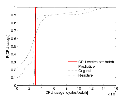
In Figure 8, we plot the Cumulative Distribution Function (CDF) of the CPU cycles
consumed to process a single batch (i.e., the service time per batch). Recall that
batches represent 100ms resulting in 3 × 10⁸ cycles available to process each
batch.
The figure shows that the predictive system is stable. As expected, sometimes the
limit of available cycles is slightly exceeded owing to the buffer discovery
algorithm presented in Section 6.1. The CDF also indicates good CPU usage
between 2.5 and 3 × 10⁸ cycles per batch, i.e., the system is rarely under- or
over-sampling.
On the contrary, the service time per batch when using the original and reactive
approaches is much more variable. It is often significantly larger than the
batch interarrival time, with a probability of exceeding the available cycles
greater than 30% in both executions. This leads to very unstable systems that
introduce packet drops without control, even of entire batches. Figure 8
shows that more than 20% of the batches in the original execution, and
around 5% in the reactive one, are completely lost (i.e., service time equal to
zero).
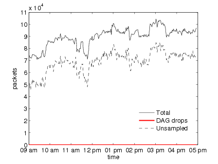
Figure 9 illustrates the impact of exceeding the available cycles on the input
stream. The line labeled ‘DAG drops’ refers to the packets dropped on the network
capture card due to full memory buffers (results are averaged over one second). These
drops are uncontrolled and contribute most to the errors in the query results. The
line ‘unsampled’ counts the packets that are not processed due to packet or flow
sampling.
Figure 9(a) confirms that, during the 8 hours, not a single packet was lost by the
capture card when using the predictive approach. This result indicates that the
system is robust against overload.
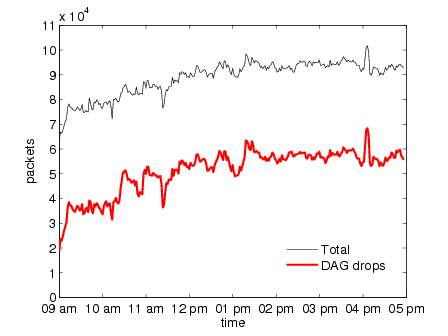
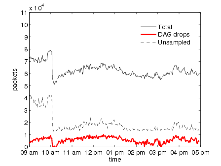
Figures 9(b) and 9(c) show instead that the capture card drops packets
consistently during the entire execution6. The number of drops in the original
approach is expected given that the load shedding scheme is based on dropping
packets on the input interface. In the case of the reactive approach instead, the drops
are due to incorrect estimation of the cycles needed to process each batch. The
reactive system bases its estimation on the previous batch only. In addition, it must
be noted that traffic conditions in the reactive execution were much less adverse,
with almost half of traffic load, than in the other two executions (see Table 5). It is
also interesting to note that when the traffic conditions are similar in all executions
(from 9am to 10am), the number of unsampled packets plus the packets
dropped by the reactive system is very similar to the number of unsampled
packets by the predictive one, in spite of that they incur different processing
overheads.
|
| Figure 9: | Link load and packet drops during the evaluation of each load
shedding method |
|
7.4 Accuracy
We modified the source code of five of the seven queries presented in Table 1, in
order to allow them to estimate their unsampled output when load shedding is
performed. This modification was simply done by multiplying the metrics
they compute by the inverse of the sampling rate being applied to each
batch.
We did not modify the pattern search and trace queries, because no standard
procedure exists to recover their unsampled output from sampled streams and to
measure their error. In this case, the error should be measured in terms of the
application that uses the output of these two queries. As discussed in Section 6.2, we
also plan to support other load shedding mechanisms for those queries that are not
robust against sampling.
In the case of the link-count, flows and high-watermark queries, we measure the
relative error in the number of packets and bytes, flows, and in the high-watermark
value, respectively. The error of the application query is measured as a weighted
average of the relative error in the number of packets and bytes across all
applications. The relative error is defined as |1 - |, where the actual
value is obtained from the complete packet trace, and all queries use packet sampling
as load shedding mechanism, with the exception of the flows query that uses flow
sampling.
|, where the actual
value is obtained from the complete packet trace, and all queries use packet sampling
as load shedding mechanism, with the exception of the flows query that uses flow
sampling.
In order to measure the error of the top destinations query, we use the detection
performance metric proposed in [2], which is defined as the number of misranked
flow pairs, where the first element of a pair is in the top-10 list returned by the query
and the second one is outside the actual top-10 list. In this case, we selected packet
sampling as load shedding mechanism [2].
Table 6 presents the error in the results of these five queries averaged across all
the measurement intervals. We can observe that, although our load shedding system
introduces a certain overhead, the error is kept significantly low compared to the two
reactive versions of the CoMo system. Recall that the traffic load in the
reactive execution was almost half of that in the other two executions. Large
standard deviation values are due to long periods of consecutive packet drops in
the alternative systems. It is also worth noting that the error of the top
destinations query obtained in the predictive execution is consistent with that
of [2].
|
|
|
| | Query | predictive | original | reactive |
|
|
|
| | application (pkts) | 1.03% ±0.65 | 55.38% ±11.80 | 10.61% ±7.78 |
|
|
|
| | application (bytes) | 1.17% ±0.76 | 55.39% ±11.80 | 11.90% ±8.22 |
|
|
|
| | flows | 2.88% ±3.34 | 38.48% ±902.13 | 12.46% ±7.28 |
|
|
|
| | high-watermark | 2.19% ±2.30 | 8.68% ±8.13 | 8.94% ±9.46 |
|
|
|
| | link-count (pkts) | 0.54% ±0.50 | 55.03% ±11.45 | 9.71% ±8.41 |
|
|
|
| | link-count (bytes) | 0.66% ±0.60 | 55.06% ±11.45 | 10.24% ±8.39 |
|
|
|
| | top destinations | 1.41 ±3.32 | 21.63 ±31.94 | 41.86 ±44.64 |
|
|
|
| | |
| Table 6: | Breakdown of the accuracy error of the different load shedding
methods by query (mean ± stdev) |
|
7.5 Overhead
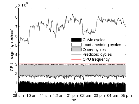
Figure 10 presents the CPU usage during the predictive execution, broken down by
the three main tasks presented in Section 6 (i.e., como_cycles, query_cycles and
ps_cycles + ls_cycles). We also plot the cycles the system estimates as needed to
process all incoming traffic (i.e., pred_cycles). From the figure, it is clear that the
system is under severe stress because, during almost all the execution, it
needs more than twice the cycles available to run our seven queries without
loss.
The overhead introduced by our load shedding system (ps_cycles + ls_cycles) to
the normal operation of the entire CoMo system is reasonably low compared to the
advantages of keeping the CPU usage and the accuracy of the results well under
control. Note that in Section 5.4 the cost of the prediction subsystem is measured
without performing load shedding. This resulted in an overall processing cost
similar to the pred_cycles in Figure 10 and therefore in a lower relative
overhead.
While the overhead incurred by the load shedding mechanism itself (ls_cycles) is
similar in any load shedding approach, independently of whether it is predictive or
reactive, the overhead incurred by the prediction subsystem (ps_cycles) is particular
to our predictive approach. As discussed in Section 5.4, the bulk of the prediction
cost corresponds to the feature extraction phase, which is entirely implemented
using a family of memory-efficient algorithms that could be directly built in
hardware [15]. Alternatively, this overhead could be reduced significantly by
applying sampling in this phase or simply reducing the accuracy of the bitmap
counters.
Finally, our current implementation incurs additional overhead, since it is not
completely integrated with the rest of the CoMo system to minimize the number of
modifications in the core platform. An alternative would be to merge the filtering
process with the prediction in order to avoid scanning each packet twice (first to
apply the filter and then to extract the features) and to share computations between
queries that share the same filter rule. Better integration of the prediction and load
shedding subsystem with the rest of the CoMo platform is part of our on-going
work.
8 Conclusions and Future work
Effective load shedding methods are now indispensable to allow network monitoring
systems to sustain the rapidly increasing data rates, number of users and complexity
of traffic analysis methods.
In this paper, we presented the design and evaluation of a system that is able to
predict the resource requirements of arbitrary and continuous traffic queries,
without having any explicit knowledge of the computations they perform.
Our method is based on extracting a set of features from the traffic streams
to build an on-line prediction model of the query resource requirements,
which is used to anticipate overload situations and effectively control the
overall system CPU usage, with minimum impact on the accuracy of the
results.
We implemented our prediction and load shedding scheme in an existing network
monitoring system and deployed it in a research ISP network. Our results show that
the system is able to predict the resources required to run a representative set of
queries with small errors. As a consequence, our load shedding scheme can effectively
handle overload situations, without packet loss, even during long-lived executions
where the monitoring system is under severe stress. We also pointed out a
significant gain in the accuracy of the results compared to two versions of the
same monitoring system that use a non-predictive load shedding approach
instead.
In the paper, we have already identified several areas of future work. In
particular, we are currently working on adding other load shedding mechanisms to
our system (e.g., lightweight summaries) for those queries that are not robust
against sampling. We also intend to develop smarter load shedding strategies
that allow the system to maximize its overall utility according to utility
functions defined by each query. Finally, we are interested in applying similar
techniques to other system resources such as memory, disk bandwidth or storage
space.
9 Acknowledgments
This work was funded by a University Research Grant awarded by the Intel Research
Council, and by the Spanish Ministry of Education (MEC) under contract
TEC2005-08051-C03-01 (CATARO project). Authors would also like to thank the
Supercomputing Center of Catalonia (CESCA) for allowing them to collect the
packet traces used in this work.
References
[1] Bar-Yossef, Z., Jayram, T. S., Kumar, R., Sivakumar, D., and
Trevisan, L. Counting distinct elements in a data stream. In Proc. of
Intl. Workshop on Randomization and Approximation Techniques (2002),
pp. 1–10.
[2] Barakat, C., Iannaccone, G., and Diot, C. Ranking flows from
sampled traffic. In Proc. of CoNEXT (2005), pp. 188–199.
[3] Barlet-Ros, P., Iannaccone, G., Sanjuŕs-Cuxart,
J., Amores-López, D., and Solé-Pareta, J. Predicting resource usage
of arbitrary network traffic queries. Tech. rep., Technical University of
Catalonia, 2006.
http://loadshedding.ccaba.upc.edu/prediction.pdf.
[4] Bloom, B. H. Space/time trade-offs in hash coding with allowable
errors. Commun. ACM 13, 7 (1970), 422–426.
[5] Carney, D., et al. Monitoring streams - a new class of data
management applications. In Proc. of Intl. Conf. on Very Large Data Bases
(2002), pp. 215–226.
[6] Carter, J. L., and Wegman, M. N. Universal classes of hash
functions. Journal of Computer and System Sciences 18, 2 (1979), 143–154.
[7] Chandrasekaran, S., et al. TelegraphCQ: Continuous dataflow
processing of an uncertain world. In Proc. of Conf. on Innovative Data
Systems Research (2003).
[8] Chi, Y., Yu, P. S., Wang, H., and Muntz, R. R. Loadstar: A
load shedding scheme for classifying data streams. In Proc. of SIAM Intl.
Conf. on Data Mining (2005).
[9] Cisco Systems. NetFlow services and applications. White Paper,
2000.
[10] Dillon, W. R., and Goldstein, M. Multivariate Analysis: Methods
and Applications. John Wiley and Sons, 1984.
[11] Duffield, N. Sampling for passive internet measurement: A review.
Statistical Science 19, 3 (2004), 472–498.
[12] Duffield, N., Lund, C., and Thorup, M. Flow sampling under
hard resource constraints. In Proc. of ACM Sigmetrics (2004), pp. 85–96.
[13] Endace. http://www.endace.com.
[14] Estan, C., Keys, K., Moore, D., and Varghese, G. Building a
better NetFlow. In Proc. of ACM Sigcomm (2004), pp. 245–256.
[15] Estan, C., Varghese, G., and Fisk, M. Bitmap algorithms for
counting active flows on high speed links. In Proc. of ACM Sigcomm Conf.
on Internet Measurement (2003), pp. 153–166.
[16] Iannaccone, G. Fast prototyping of network data mining
applications. In Proc. of Passive and Active Measurement (2006).
[17] Intel Corporation. The IA-32 Intel Architecture Software
Developer’s Manual, Volume 3B: System Programming Guide, Part 2. 2006.
[18] Keys, K., Moore, D., and Estan, C. A robust system for accurate
real-time summaries of internet traffic. In Proc. of ACM Sigmetrics (2005),
pp. 85–96.
[19] L’Anella Científica (The Scientific Ring).
http://www.cesca.es/en/comunicacions/anella.html.
[20] NLANR: National Laboratory for Applied Network
Research.
http://www.nlanr.net.
[21] Press, W. H., Teukolsky, S. A., Vetterling, W. T., and
Flannery, B. P. Numerical Recipes in C: The Art of Scientific
Computing, 2nd ed. 1992.
[22] Reiss, F., and Hellerstein, J. M. Declarative network monitoring
with an underprovisioned query processor. In Proc. of Intl. Conf. on Data
Engineering (2006), pp. 56–67.
[23] Tatbul, N., et al. Load shedding in a data stream manager. In
Proc. of Intl. Conf. on Very Large Data Bases (2003), pp. 309–320.
[24] Welsh, M., Culler, D. E., and Brewer, E. A. SEDA: An
architecture for well-conditioned, scalable internet services. In Proc. of
ACM Symposium on Operating System Principles (2001), pp. 230–243.
[25] Whang, K.-Y., Vander-Zanden, B. T., and Taylor, H. M.
A linear-time probabilistic counting algorithm for database applications.
ACM Trans. Database Syst. 15, 2 (1990), 208–229.
[26] Yu, L., and Liu, H. Feature selection for high-dimensional data: A
fast correlation-based filter solution. In Proc. of Intl. Conf. on Machine
Learning (2003), pp. 856–863.
Notes
1The choice of 100ms is somewhat arbitrary. Our experimental results indicate that 100ms
represents a good trade-off between accuracy and delay with the traces of our dataset. We
leave the investigation on the proper batch duration for future work.
2A description of the queries used in our experiments can be found in [3]. The actual source
code of all queries is also publicly available at http://como.sourceforge.net.
3It is possible that the CPU usage of other queries may exhibit a non-linear relationship
with the traffic features. A possible solution in that case is to define new features computed
as non-linear combinations of simple features.
4Note that the values of some predictors may become very similar under special traffic
patterns. For example, the number of packets and flows can be highly correlated under a
SYN-flood attack.
5The source code of the prediction and load shedding system is available at
http://loadshedding.ccaba.upc.edu. The CoMo monitoring system is also available at
http://como.sourceforge.net.
6The values are a lower bound of the actual drops, because the loss counter present in the
DAG records is only 16-bit long.