Security '05 Paper    [Security '05 Technical Program]

On the Effectiveness of Distributed Worm Monitoring

Moheeb Abu Rajab

Fabian Monrose

Andreas Terzis

Computer Science Department
Johns Hopkins University

{moheeb,fabian,terzis}@cs.jhu.edu

Abstract:

Distributed monitoring of unused portions of the IP address space holds the promise of providing early and accurate detection of high-profile security events, especially Internet worms. While this observation has been accepted for some time now, a systematic analysis of the requirements for building an effective distributed monitoring infrastructure is still missing. In this paper, we attempt to quantify the benefits of distributed monitoring and evaluate the practicality of this approach. To do so we developed a new worm propagation model that relaxes earlier assumptions regarding the uniformity of the underlying vulnerable population. This model allows us to evaluate how the size of the monitored address space, as well the number and locations of monitors, impact worm detection time. We empirically evaluate the effect of these parameters using traffic traces from over 1.5 billion suspicious connection attempts observed by more than 1600 intrusion detection systems dispersed across the Internet.

Our results show that distributed monitors with half the allocated space of a centralized monitor can detect non-uniform scanning worms in half the time. Moreover, a distributed monitor of the same size as a centralized monitor can detect the worm four times faster. Furthermore, we show that even partial knowledge of the vulnerable population density can be used to improve monitor placement. Exploiting information about the location of the vulnerable population leads, in some cases, to detection time that is seven times as fast compared to random monitor deployment.

1 Introduction

Attacks from malware, such as network worms, pose without a doubt, one of the most significant threats to the livelihood of the Internet [1]. For the most part, these attacks are countered today by manual, collaborative efforts by network operators. Typically, operators monitor traffic through their networks using network management tools, and report any suspicious traffic surges to mailing lists (e.g., NANOG [16]) to alert other operators about the active spread of a new malware strain. Operators managing different networks then apply rudimentary traffic filters to block suspected malicious traffic or to drop all packets coming from offending sources.

In an effort to establish a broader knowledge base for analyzing suspicious traffic, there has been a recent movement towards widespread participation in centralized repositories like DShield [7]. Over the past year, DShield's repository, for example, has observed a steady increase in the submission of intrusion logs by volunteering networks from all over the globe. For the most part, these repositories correlate events across the supplied reports, and release daily summaries of malicious traffic activity (e.g., top offenders) that can be used to update network filtering rules.

While these approaches can provide some level of defense, the fact that information is not generated and disseminated in a timely fashion limits the value of these approaches. Recent studies [19,20] have shown that worms can reach saturation in just a few minutes, rendering these solutions of little practical value in detecting and containing such outbreaks. To address this, a number of proposals have surfaced aiming to facilitate the development of an automated distributed infrastructure of network monitors [2,5,22]. In these proposals, each monitor collects traces of potentially malicious traffic and exchanges information with the other members of the infrastructure so that a broader view of the attack can be created. The general thinking here has been that an effective automated early warning strategy could hopefully be used to leverage automatic containment solutions.

Unfortunately, while the recent interest in creating distributed monitoring systems is indeed a positive development, little is known about how such a system should be deployed in the most effective way. Specifically, numerous questions arise regarding the size, number, and location of such monitors. Our focus in this paper is to explore the feasibility of such an approach, and investigate a number of criteria that impact the effectiveness of a distributed monitoring architecture. Furthermore, we examine what would be the relative improvement in the system's detection time if the density of the vulnerable host population was known. While we understand that knowing this distribution a priori is fairly difficult, and some may argue infeasible, we contend that the answer to this question is interesting nonetheless. For one, if given knowledge (or some approximation thereof) of the distribution of vulnerable hosts still provides no substantial improvement in detection speed, then monitors can be deployed anywhere in the IP address space. If, on the other hand, such knowledge provides substantial benefits, this may imply that network operators will need to tackle ways to estimate this distribution in order for a distributed monitoring system to be of any practical significance.

To pursue our goals, we extend existing worm models to more accurately reflect the spreading behavior of worms. While several models for worm propagation have been proposed to date (e.g. [4,11]), we believe these models make assumptions that significantly distort the models' view of the actual worm behavior. Most notably, the previous models are lacking in that they do not make use of the density of vulnerable hosts or incorrectly assume that such hosts are uniformly distributed across the address space. By contrast, our approach takes into account the distribution of the vulnerable population over the address space. Indeed, deriving models that can take advantage of this knowledge is a non-trivial task, particularly when studying the behavior of non-uniform scanning worms such as Code Red II and Nimda. In fact, deriving such a model has been viewed as a challenging problem in its own right [19].

Using our extended model, we evaluate different aspects of distributed monitoring using simulations driven by real data traces. Our primary data set, obtained from DShield [7], is a collection of intrusion detection logs from more than 1600 networks from around the globe. The collected traces span a period of 3 months and contain more than 1.5 billion malicious connection attempts.

CONTRIBUTIONS: This paper makes three main contributions: (1) we propose an extension to current worm models that does not assume the distribution of vulnerable hosts over the IP address space is uniform. As a result, our model reflects the dynamics of non-uniform scanning worms more accurately, (2) we derive a model for the detection capability of distributed monitors, and (3) we use this model to evaluate the relative performance of different distributed monitor configurations. These configurations differ in the number and size of individual monitors as well as in their knowledge of the vulnerable population distribution.

The rest of the paper is organized as follows: In Section 2 we summarize previous work related to worm modeling and detection. Section 3 presents the distribution of vulnerable hosts derived from collected traces. We present our extended model in Section 4 and provide metrics for evaluating the detection capability of a distributed monitoring system in Section 5. We use this observation model as a basis for the experiments in Section 6. We conclude in Section 7 with some remarks and future work.

2 Related Work

2.1 Worm Modeling

Over the last few years, several approaches have been suggested for modeling the spread of worms (e.g, [4,19,25,26]). In [19] Staniford et al. used the classic epidemic model [11] to model the spreading behavior of the CodeRed worm [9]. However, the epidemic model is unable to capture the spreading behavior of non-uniform scanning worms such as Nimda [12] and Code Red II [15]. Moreover, as shown by Chen et al. the epidemic model over-estimates the infection speed as it does not consider the joint probability of a host being scanned by different sources at the same time [4]. A more promising probabilistic model, called the Analytical Active Worm Propagation model (AAWP) was proposed in [4]. In this model the probability, $P_{(m,n)}$, that a vulnerable host will receive $m$ scans from a total of $n$ sent by $n_i$ infected hosts at time tick $i$, is modeled by a binomial random variable with probability of success $p = 1/2^{32}$ and number of trials (i.e., scans) $n=sn_i$ where $s$ is the average scanning rate of a single infected host (The notation is given in Table 1). Let $P_i$ be the probability that a vulnerable host will be infected at time tick $i$. Then, $P_i$ is the probability that the host will be scanned at least once by any infected host, therefore:

$$P_i = 1-P_{(0,n)} = 1 - \left(1- \frac{1}{2^{32}}\right)^{sn_i}$$ (1)

From Eq. (1), the expected number of infected hosts at time tick $i+1$ can be expressed as:

$$n_{i+1} = n_i + \big(V - n_i\big) \Bigg[1- \big( 1- \frac {1}{2^{32}}\big)^{sn_i}\Bigg]$$ (2)

Equation (2) models the behavior of uniform scanning worms like Code Red, where all vulnerable hosts have an equal probability of being scanned by an infected host regardless of their location relative to that infected host.

For non-uniform scanning worms, Chen et al [4] proposed an extension to the above model by considering the preferential scanning strategy of non-uniform worms towards local /16 and /8 subnets. However, as is the case with most previous work, the authors assume that the vulnerable population is uniformly distributed over the IP space--which, as we show later, is not a valid assumption. Recently, Gu et. al. [10] acknowledge that the earlier assumption in [4] is problematic, and attempt to address this by instead assuming that vulnerable hosts are uniformly distributed only in the assigned IPv4 space (i.e., about $1/4$ of the IPv4 space according to [21,24]). However, this also is an over-simplification, as there is no reason to believe that the density of hosts within the allocated address space is uniform. In fact, as we show in Section (3), our empirical data suggests that host density diverts significantly from the uniform distribution. Therefore, we believe that completely relaxing this assumption makes the most sense at this point, as the actual distribution of vulnerable hosts has significant implications on the model's accuracy. In this work, we propose an improvement to prior models by incorporating the distribution of the vulnerable population over the address space, and we show the profound implications of this factor on the spreading behavior of non-uniform scanning worms.

Table 1: Worm Model Notation.

$V$	Total number of vulnerable hosts
$n_i$	Number of infected nodes at tick $i$
$P_{(m,n)}$	The probability that a vulnerable host
	receives $m$ out of $n$ total scans
$P_{i}$	The probability that a vulnerable host
	is infected at time tick $i$
$s$	Average scan rate (scans/time tick)
	per infected node
$p_{0}$	Probability that a worm instance scans a random address
$p_{8}$	Probability that a worm instance scans an address
	within the same $/8$ prefix
$p_{16}$	Probability that a worm instance scans an address
	with the same $/16$ prefix
$v^j$	Number of vulnerable machines in the $j$-th /16 subnet
$b_i^j$	Number of infected nodes in the $j$-th $/16$ subnet
	at time $t_i$
$k_i^j$	Aggregate number of scans within the $j$-th $/16$
	subnet at time $t_i$
$b_i^{(/8)}$	Number of infected hosts in the common
	/8 subnet as the victim host.

2.2 Monitoring

For the last few years researchers at CAIDA [14] have used traffic monitors over unused address space (also called telescopes or traffic sinks) to monitor large scale network security events and provide forensic analysis of such outbreaks. Unfortunately, while valiant in their efforts, for non-uniform scanning worms (e.g, CodeRed-II), CAIDA's telescope remains unable to glean reliable information about the worm activity as the telescope only observes part of the address space being preferentially scanned by such worms (e.g, the 1/8 scanning component for the case of CodeRed-II [15]).

In [2,5] Bailey, Cooke, et. al. propose a distributed monitoring system using a set of monitors of varying sizes provided by a collection of ISPs and academic institutions. In that work, a central aggregator is used to combine information from different monitors and to provide relevant summaries of any outstanding security event. Though that work embodies an important first step towards achieving a realistic distributed monitoring infrastructure, the interplay between size, number, and deployment of monitors and its effect on detection capability was not addressed. The work presented here will hopefully shed light on these issues and better assist deployment strategies for use in [2].

Our work is also distantly related to that of the DOMINO system [22] where the benefits of combining reports from different intrusion detection systems were explored. However, our work differs significantly in its goal and scope from DOMINO--for one, while DOMINO's evaluation is primarily based on combining intrusion detection logs from different operational networks, our work is focused on evaluating the benefit (and feasibility) of collectively monitoring unused IP space distributed throughout the Internet. Moreover, unlike [22], we explore the effect of size and placement of distributed monitors on improving the system's overall detection time.

3 Population Distribution

A central thesis of this paper is evaluating whether a priori knowledge of the distribution of vulnerable hosts can improve the overall rate at which an outbreak is detected. As mentioned earlier, prior models, including the AAWP model [4] and its extensions, make the simplifying assumption that the vulnerable population is uniformly distributed over the (used) IP space. Here, we question the validity of this assumption based on collected data.

Data:

Our data consists of three months worth of IDS logs collected by DShield [7]. The logs were volunteered by more than 1600 Intrusion Detection Systems distributed around the globe, and contain more than 1.5 billion connection attempts from nearly 32 million unique sources. Table 2 contains a summary of the relevant information.

Table 2: Summary of the DShield data

Total Unique sources	31,864,871
Total number of connections	1,509,619,146
Most attacked ports
Port	unique sources
Port 445	11,889,416
Port 135	5,139,751
Port 80	632,472

Since our traffic logs are obtained from IDS reports, it is safe to assume that they represent unwanted traffic. This traffic originates either from compromised hosts or active scanners.¹ We further filter the data by considering only sources attempting connections to ports 80, 135, and 445. We chose these ports because they are targeted by many well-known worms (e.g. CodeRed, Nimda, and MS Blaster). We assume that all connection attempts to these ports originate from previously compromised hosts attempting to transfer the infection to other hosts by scanning the address space. Therefore, we assume that the collected set of source IP addresses attempting connections to one of the above specified ports, is the set of hosts that were originally vulnerable to (and subsequently infected by) a worm instance. There is a caveat, however, with identifying hosts based solely on their IP addresses: because DHCP is heavily used, hosts may be assigned different addresses over time. Indeed, Moore et. al. [15] argue that IP addresses are not an accurate measure of the spread of a worm on time-scales longer than 24 hours. Unfortunately, without a better notion at hand, we proceed to use IP addresses to identify hosts, but keep this observation in mind.

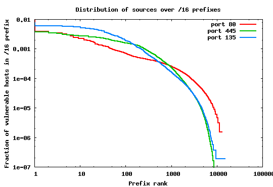
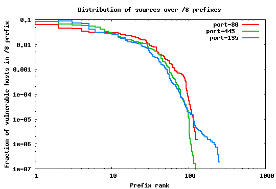
We group the IP addresses in each of the three sets according to two granularities: (i) in /16 prefixes, and (ii) in /8 prefixes. We chose these two groupings because they are important from the perspective of worm spreading behavior. Specifically, it is known that many examples of popular worms (e.g. [6,8,12]) use localized target selection algorithms targeting hosts with different scanning probabilities applied on the /16 and /8 prefix boundaries.

Figure 1: Percentage of malicious sources per /16 prefix

Figure 2: Percentage of malicious sources per /8 prefix

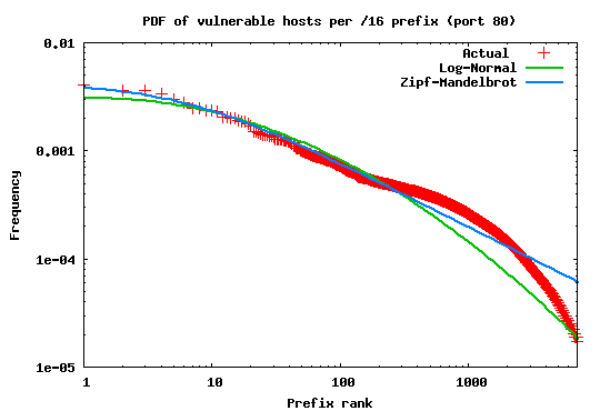
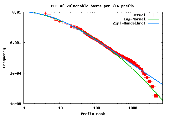
The rank plots in Figures 1 and 2 show the percentage of malicious sources in each /16 and /8 prefix over the total number of sources. It is clear that in both cases the population distribution is far from being uniform. This result can be interpreted intuitively by the fact that the utilization of the address space is not uniform--some portions of the space are unallocated, large prefixes are owned by corporations with small number of hosts, while others (belonging to edge ISPs, for example) may contain a large number of less protected client machines.

In fact, the relatively straight lines in these log-log plots indicate that the distributions of vulnerable hosts among prefixes follow a power law. To better explore this conjecture, we fit the curve representing sources attempting connections to port 80 to well known power-law probability distributions. Figure 3 shows the result of this fitting. As the graph shows the source distribution best fits a Log-normal with parameters ($s=2.7$) and ($m=7.5$) ².

Figure 3: Fit of vulnerable host population probability density function to known probability distributions

To further validate this observation we performed a similar evaluation on a traffic log of the Witty worm [18] obtained from CAIDA [3]. We applied the same aggregation methodology described above on the set of unique sources of scans detected by CAIDA's /8 network telescope. These sources are, without any doubt, infected hosts attempting to spread the worm infection to other potential victims. Figure 4 shows that the heavy tailed tendency in the infected population distribution is even more pronounced. Again, the trend appears to closely fit a Log-normal distribution with parameters ($s=2.67$) and ($m=6.1$).

Figure 4: Fit of Witty worm infected hosts probability density function to known probability distributions.

These results provide clear evidence that the vulnerable population distribution is far from being uniformly distributed. In the next sections we develop an extended worm model that incorporates this observation and then use this model to evaluate various aspects of distributed monitoring. Our subsequent analyzes are based on the DShield data set as it is not tied to any particular event and it is therefore more general.

4 Extended Worm Propagation Model

First, we derive an extended model based off the AAWP model given in [4]. Our extended model allows us to account for the non-uniformity in the distribution of the vulnerable population, and later we show how this extension significantly impacts the predictions made by previous models specifically for the case of non-uniform scanning worms.

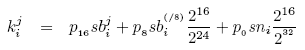
For a non-uniform scanning worm with a Nimda-like scanning behavior, to compute the expected number of infected hosts at time tick $i+1$, we first compute the expected number of incoming scans into each /16 prefix at time tick $i$ and use the result to predict the number of infected hosts in each /16 subnet at time step $i+1$. Let $k^{j}_i$ denote the total number of incoming scans into the $j^{th}$ /16 prefix at time tick $i$. Then $k^{j}_i$ is the sum of the scans originating from infected hosts within the same /16 prefix (each scanning with rate $p_{_{16}}s$, where $p_{_{16}}$ is the probability that the worm scans hosts within the same /16 prefix as the infected host), scans from infected hosts within the encompassing /8 subnet (each scanning with a rate $p_{_8}s$, where, $p_{_{8}}$ is the probability that the worm scans hosts within the same /8 prefix as the infected host), and scans originating from infected hosts from anywhere in the address space (each scanning with rate $p_{_{0}}s$, where, $p_{_{0}}$ is the probability the worm scans a host selected at random from the whole IP space). Therefore, $k^j_i$ can be expressed as follows:

where $s$ denotes the average scanning rate of the worm, $b_i^j$ the number of infected hosts in the $j^{th}$ /16 aggregate at time tick $i$, $b_i^{^{(/8)}}$ the number of infected hosts in all /16 subnets within the same /8 prefix. Then, using a similar derivation as in Equation (2), the expected number of infected hosts per /16 subnet at time tick $i+1$ can be expressed as:

$$b_{i+1}^j = b_i^j + (v_i - b_i^j) \Bigg[1- \Big( 1- \frac {1}{2^{^{16}}}\Big)^{k_i^j}\Bigg]$$ (5)

The expected total number of infected hosts by the worm at time tick $i+1$ is simply the sum of the infected hosts in all possible $2^{16}$ /16 prefixes:

$$n_{i+1} = \sum_{j=1}^{2^{{^{16}}}} b_{i+1}^j$$ (6)

Figure 5: Infection speed predicted by the extended model for a uniform and non-uniform scanning worm when the vulnerable hosts are uniformly distributed.

REMARK: We note that our decision to study a worm with a Nimda-like target selection algorithm is for illustrative purposes only. The analysis presented here can be generalized to other classes of worms that apply different scanning strategies on prefix boundaries other than the /16 and /8 boundaries. However, preferentially scanning at the /16 and /8 prefix boundaries is considered a successful strategy and a widely used practice by most non-uniform scanning worms [6,8,12]; therefore a Nimda-like worm behavior serves our purpose well.

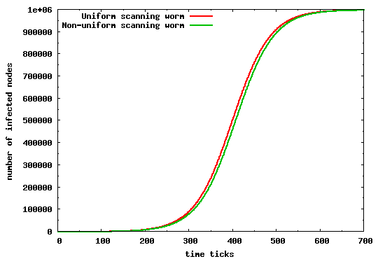
To validate the extended model we compare it to the original AAWP model, using the same set of assumptions and simulation parameters as those used in [4]. For completeness, we restate these parameters in Table 3. We compare our model for both a uniform and non-uniform scanning worm. Clearly, if our model is correct we should arrive at an identical propagation evolution as that in [4]. Figure 5 depicts the infection propagation in both scenarios. Our results are identical to those found in [4], and (we believe) lead to an incorrect conclusion--that a uniform scanning worm propagates faster than its non-uniform counterpart.

Table 3: Simulation Parameters

Number of Vulnerable hosts	1,000,000
Scanning rate per infected hosts $s$	100 scans/tick
Size of initial Hit List	100 randomly distributed
	over the populated IP space
Scanning probabilities	$p_{_{16}}$	$p_{_{8}}$	$p_{_{0}}$
Nimda-Like	0.5	0.25	0.25
Uniform scanning	0	0	1

To see why this is not the case, we demonstrate the impact of the vulnerable population distribution on the results predicted by the model. We do so by using the set of sources attempting suspicious connections to port 80 extracted from the DShield data set. Again, we apply the same simulation parameters from Table 3, but with 632,472 sources (i.e., the number of sources in the DShield data) attempting connections to port 80. We use this data set to drive our simulation model under two different scenarios. In the first scenario we ignore the actual locality of hosts and assume that they are evenly distributed over the IP space, while in the latter we use the actual distribution of sources per /16 prefix extracted from the DShield data set.

The difference in propagation speed between these two cases is dramatic; the leftmost line in Figure 6 depicts the infection evolution of the worm with an underlying population distribution inferred from DShield traces, while the rightmost line shows the evolution of the infection based on the uniform population distribution assumption. The AAWP model would predict that the non-uniform scanning worm would be able to infect the whole population after 1000 time ticks from the breakout. However, under the more realistic distribution derived from the actual data set, we see that a non-uniform worm would infect the whole vulnerable population in less than 200 time ticks -- 5 times faster than the previous case. Clearly, the significant discrepancy between the two predictions underscores the fact that the underlying locality distribution of the vulnerable population is an important factor that can not be overlooked especially when modeling non-uniform scanning worms.

Figure 6: Impact of population distribution on non-uniform worm propagation.

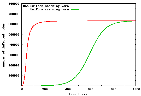
Finally, we revisit the claim that a uniform scanning worm propagates faster than its non-uniform counterpart. We do so by comparing the propagation behavior of a uniform scanning worm to a non-uniform scanning worm but with vulnerable population distribution derived from the DShield traces. As Figure 7 illustrates, a non-uniform scanning worm can spread significantly faster than a uniform scanning worm with the same average scanning rate and same vulnerable population size. The results are enough to warrant restatement: that a simply designed non-uniform scanning worm would reach saturation much faster than one with uniform scanning characteristics. Intuitively, worm instances within heavily populated subnets, quickly infect all vulnerable hosts within these subnets by applying a biased target selection algorithm towards these hosts; recall that a Nimda worm instance sends 75% of its scans to hosts within the same /16 prefix and same /8 prefix. This behavior exploits the power law distribution shown in Figure 1, where the majority of hosts are in a relatively low number of heavily populated prefixes. Therefore, even a single infected host within such prefixes is enough to spread the infection to a large number of vulnerable hosts in a very short time. This explains the sharp initial increase in the number of infections for the non-uniform scanning worm.

These above observations support Staniford et. al.'s earlier conjecture that a non-uniform scanning worm would spread faster than its uniform counterpart [19]. Also, as we show later, this leads to a set of important design considerations for a distributed worm monitoring system, especially as it relates to the location, number, and size of the monitors.

Figure 7 : Extended Model: Number of infected nodes vs. time for uniform and non-uniform scanning worms.

In the following sections we use this extended model to estimate the detection time of different distributed monitor configurations.

5 Evaluating Distributed Worm Monitoring

Over the last few years, a number of research projects have proposed the use of network monitors (also called telescopes [14] or traffic sinks) for forensic analysis of worms, as well as for estimating the prevalence of security events such as DDoS attacks [13,21,23]. However, several questions regarding the practicality of distributed monitoring and its pertinent design considerations such as required number, size and deployment considerations have been left unanswered. To answer such questions, we introduce an observation model that measures the detection capability of a distributed monitoring system. Specifically, the model computes the probability, $P_d$, that an instance of the worm is observed by any monitor in the system. We then use this probability to derive a detection metric that computes the expected time elapsed before the monitoring system detects (with a certain confidence level) a worm instance.

5.1 A Distributed Monitoring Model

Table 4: Monitor modeling parameters.

$V$	Total number of vulnerable hosts
$s$	Average scan rate (scans/time tick)
	per infected node
$S$	The total size of address space covered by monitors
$S_c$	The IP space size scanned by an infected node
	at different layers of the hierarchy
$S^{l}$	The monitor size in layer $l$ relative to
	an infected host
$S^{\scriptscriptstyle(/16)}$	Monitor size within the same /16 subnet as an
	infected host
$S^{\scriptscriptstyle(/8)}$	Monitor size within the same /8 subnet as an
	infected host
$P_{d}$	The probability that a certain scanner is detected by the
	distributed monitoring system
$P_{r}$	The probability that a certain scanner is detected by the
	distributed monitoring system up to a detection time $t_d$
$p_{\scriptscriptstyle l}$	The preferential worm scanning probability applied
	to the common space $S_c$
$P_{e}^{l}$	The probability that a monitor exists in the
	logical layer $l$ relative to an infected host
$P_{e}^{\scriptscriptstyle(/16)}$	The probability that a monitor exists within the
	/16 subnet of an infected host
$P_{e}^{\scriptscriptstyle(/8)}$	The probability that a monitor exists within the
	/8 subnet as an infected host

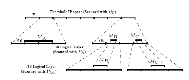
The notation we use is summarized in Table (4). To facilitate computing $P_d$, we organize monitors into a logical hierarchy. Each layer in the hierarchy can ``see'' scans with a certain probability according to its location in the address space (relative to an infected host) and according to the worm preferential scanning strategy. In the case of Nimda, the distributed monitoring system can be logically divided into a three-tier hierarchy. Figure 8 shows an example of this logical hierarchy. In our example there are three monitors: $M_{\scriptscriptstyle A}$ of size /9, $M_{\scriptscriptstyle B}$ of size /22 and $M_{\scriptscriptstyle C}$ of size /24. $M_{\scriptscriptstyle B}$ and $M_{\scriptscriptstyle C}$ are located in two different /16 subnets but have the same /8 prefix.

Figure 8: Monitoring System Logical Layer Hierarchy.

• The first layer (/16) includes monitors within the local /16 subnets of infected hosts. If a monitor exists in this layer, it will be scanned with the worm's ``most specific'' preferential scanning probability (i.e. $p_{\scriptscriptstyle 16}$). The size $S^{\scriptscriptstyle(/16)}$ is the size of a monitor within the /16 prefix as the infected host (i.e. $M_{\scriptscriptstyle B}$ or $M_{\scriptscriptstyle C}$ in the above example).

• The second logical layer (/8) contains monitors within the /8 prefix relative to infected hosts. Such monitors will be scanned with probability $p_{\scriptscriptstyle 8}$. The size of a monitor in this layer $S^{\scriptscriptstyle(/8)}$ is the sum of all monitor sizes having the same /8 prefix. The example in Figure 8 has two logical monitors - one with size equal to the sum of $M_{\scriptscriptstyle B}$ and $M_{\scriptscriptstyle C}$ (/22 + /24) and another with size $M_{\scriptscriptstyle A}$ (/9).

• The third layer (/0) represents the aggregate of all monitors in the deployment. The size of this logical monitor $S$, is the sum of all individual monitor sizes. This monitor will be scanned with probability $p_{\scriptscriptstyle 0}$. Following our example, $S = M_{\scriptscriptstyle A} + M_{\scriptscriptstyle B} + M_{\scriptscriptstyle C}$.

To derive the detection probability $P_d$, we make the simplifying assumption that a single scan is enough to classify a source as malicious³. We also assume that any infected host is eventually detected (i.e: $P_{d_{\infty}} = 1$). Therefore, $P_d$ is formally defined as the probability that an infected host scans any monitor in the system at least once. This probability is the complement of the probability that the scanning host evades detection by monitors in all logical layers. Therefore, $P_{d}$ can be expressed as follows:

$$P_{d} = 1 - \left[\prod_{l} \Big(1- \frac{S^{l}}{S_{c}}\Big)^{p_{l} s} \right]$$ (7)

where $l$ is the index over the layers in the logical monitor hierarchy (i.e. /8, /16, and /0). $S^{l}$ denotes the relevant monitor size in layer $l$ relative to this host, $S_{c}$ is the IP space scanned by the worm instance at that layer ( i.e. /8, /16 or /0), and $p_{\scriptscriptstyle l}$ is the probability with which the worm scans layer $l$.

Then, for a non-uniform scanning worm with preferential scanning probabilities $p_{16}, p_8,$ and $p_0$, Equation (7) can be rewritten as:

$$\begin{eqnarray*} P_{d} & = & 1- \Bigg[ \Big( 1 - \frac{S^{\scriptscriptstyl... ... - \frac{S}{2^{32}} \Big) ^{p_{\scriptscriptstyle 0}\,s} \Bigg] \end{eqnarray*}$$

For a uniform scanning worm which scans the whole IP space with uniform probability (ie: $p_{\scriptscriptstyle 0}=1$, $p_{\scriptscriptstyle 8} =0$, $p_{\scriptscriptstyle 16}=0$), $P_{d}$ is simply expressed as:

$$P_{d} = 1 - \Big(1- \frac{S}{2^{32}}\Big)^{s}$$ (8)

In the following section we use our observation model to compute the expected detection time of a distributed monitoring system.

5.2 Detection Time

Arguably, the most critical indicator of the effectiveness of a worm monitoring system is its reaction time $t_d$. $t_d$ is the elapsed time from the instant an infected host sends its first scan up to the point where at least one scan from that host is detected (with a certain confidence) by any monitor in the distributed monitor deployment [14]. Using Equation (7) we define $P_r$ as the probability that the distributed monitoring system has detected a new infected host by time $t_d$. Equivalently, $P_r$ is the probability that any monitor in the system observes at least one scan from that source by the detection time $t_d$. Therefore, $P_{r}$ can be expressed as:

$$P_{r} = 1 - \prod_{i=0}^{t_d} \Bigg[ \prod_{l} \Big( 1- \frac{S^{l}}{S_{c}} \Big) ^{p_{\scriptscriptstyle l} s}\Bigg]$$ (9)

which can be simplified to:

$$P_{r} = 1 - \prod_{l} \Big(1- \frac{S^{l}}{S_{c}}\Big)^{p_{\scriptscriptstyle l} s t_d}$$ (10)

The observant reader will note that Equation (10) assumes that a monitor exists in all logical layers relative to an infected host. However, in practice the deployment of distributed monitors will not cover all such locations. For example, if we select an infected host at random, the probability that this host scans a monitored address using $p_{\scriptscriptstyle 16}$ depends on having a monitor placed within the same /16 address space as the infected host (the same applies for the other preferential scanning probabilities).

The probability that a monitor is placed near an infected host, denoted $P_e^{\scriptscriptstyle l}$, is solely defined by the distributed monitors' deployment strategy and the IP space coverage achieved by that deployment. To accommodate for this probability, we can rewrite Eq. (10) as:

$$P_{r} = 1 - \prod_{l} \Big(1- \frac{S^{l} P_e^{l}}{S_{c}}\Big)^{p_{\scriptscriptstyle l} s t_d}$$ (11)

For the case of a non-uniform scanning worm with preferential scanning probabilities $p_{16}, p_8,$ and $p_0$, $P_r$ is then given by:

$$\begin{eqnarray*} P_{r} &= &1 - \Bigg[ \Big( 1- \frac{S^{\scriptscriptstyle (/16... ...ac{S}{2^{{32}}} \Big) ^{p_{\scriptscriptstyle 0}\,s t_d} \Bigg] \end{eqnarray*}$$

where, $P_e^{\scriptscriptstyle (/16)}$ is the probability that a monitor exists in the /16 subnet of an infected host. Similarly, $P_e^{\scriptscriptstyle (/8)}$ is the probability of having a monitor within the /8 subnet of an infected host.

Our goal is to determine the expected time, $t_d$, at which the probability of detection is at a particular confidence level (e.g: 95%). Solving Eq.(11) for $t_d$ gives:

$$t_d = \frac{\log\big(1 - P_{r}\big)}{\sum_{l}\, p_{\scri... ...\Big( 1-\frac{S^{l} P_e^{\scriptscriptstyle l}}{S_{c}} \Big)}$$ (12)

Now that we have an observation model and accompanying detection metric, we proceed to evaluate the parameters and design alternatives that directly affect the detection time of distributed monitoring systems.

6 Evaluation

Our focus here is to use the model presented in Section 5 to evaluate the effectiveness of distributed monitoring. In particular, we try to evaluate to what extent does size, monitor placement, and more importantly, the number of deployed monitors impact the expected detection time.

6.1 Number and size of monitors

Moore et al. have previously highlighted that a /8 monitor has a very different view of a Code Red infection (i.e. uniform scanning worm) compared to a /16 monitor [14]. Specifically, the /8 monitor was able to provide a timely view of the worm's actual propagation, while the view from the /16 monitor was significantly delayed.

In the distributed case however, the number (and location) of monitors may be more important than aggregate size. In what follows, we compute the expected detection time $t_d$, of different monitor sizes across various combinations. To do so, we explore several deployment scenarios ranging from a total monitored address space of size /8 ($2^{24}$ addresses) down to a total size of /16 ($2^{16}$ addresses). For simplicity, each aggregate size is broken into a different number of monitors of equal sizes ⁴.

Figure 9: Detection time $t_d$ of a single infected host for different number of distributed monitors deployed randomly over the IP space. 
( $s = 10\, scans/tick$, $P_r = 0.9999$, minimum detection time is 230 time ticks)

First, we distribute monitors uniformly over the whole IP space. In order to compute $t_d$ in Eq. (12) we first need to compute $P^{l}_{e}$ for the different layers in the logical monitor hierarchy. Since we distribute monitors uniformly, the probability $P^{l}_{e}$ that a monitor exists at each layer, is simply equal to the total number of monitors divided by all the possible locations (prefixes) that these monitors can occupy.

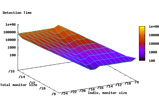
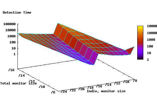
Figure 9 shows the expected detection time $t_d$ for different monitor configurations. It is clear from the graph that there is a substantial improvement in detection time associated with distributed monitoring configurations. For example, while a single /8 monitor yields a detection time of 940 time ticks, a distributed deployment of 512 /17 monitors results in a detection time of 230 ticks. During the additional detection time of 710 seconds, a worm instance can generate roughly 7100 more scans, thus infecting a larger number of vulnerable hosts before being detected. Furthermore, Figure 9 shows that configurations with a number of monitors of a certain size perform equally well, or better, than other configurations with larger total size. For instance, a distributed monitor deployment of 512 /18 monitors (i.e. /9 aggregate size) provides lower detection time (471 time ticks) than a single /8 monitor (940 time ticks).

Unfortunately, deploying monitors randomly over the IP address space is still a resource consuming proposition. The minimum detection time (230 time ticks) comes at the cost of requiring an aggregate monitor size of /8, a considerable amount of unused address space. Next, we consider whether deploying monitors in a way that takes into account the vulnerable population density over the address space can substantially reduce detection time, and if so, to what degree.

6.2 Placement of Monitors

In this section we investigate the effect of using the vulnerable population density to guide the placement of distributed monitors. To do so, we use the population distribution of sources attempting connections to port 80 inferred from the DShield data set (cf. Section 3). We understand that such information might not be available at a global scale. However, our focus here is to understand to what degree can detection time be improved given some level of knowledge about the vulnerable population.

First, we assume that we have full knowledge of the vulnerable population density over the address space and so we can deploy monitors in the most populated prefixes. In this scenario, the probability $P^{l}_e$ of having a monitor at layer $l$ of the hierarchy, is calculated in the following way: Let $C^{l}$ be the number of vulnerable hosts that have a monitor within their common prefix at layer $l$. Then, $P^{l}_e$ is equal to $C^{l}/V$, where $V$ is the size of the vulnerable population.

Figure 10: Detection time $t_d$ of a single infected host for different number of distributed monitors deployed in the top populated prefixes from DShield data. 
( $s = 10\, scans/tick$, $P_r = 0.9999$, minimum detection time is 9 time ticks )

Given $P_e$, for each size and number combination, we can compute $t_d$ directly from Equation (12). Figure 10 shows the detection time for the same set of configurations used in the previous section. It is evident that the population density aware deployment strategy can achieve significantly lower detection time. Indeed, under this scenario, a number of points are worthy of further discussion:

• The rapid decrease in detection time using individual /17 monitors reflects the effect of capturing the local preferential scanning probability for hosts within the same /16 subnet as the infected host. The minimum detection time for all aggregate sizes happens at this point because the monitoring system is able to capture the local preferential scanning behavior of the worm.

• Detection time starts to increase when monitors with individual size less than /17 are used even though the aggregate monitor size remains constant. This trend is due to the power-law distribution of vulnerable hosts. Since most vulnerable hosts are located in a relatively low number of prefixes, the benefit from covering more prefixes with a larger number of smaller monitors is overshadowed by the loss in detection capability of individual monitors.

While it would be impractical to deploy /17 monitors in the most densely populated /16 prefixes, we argue that there are a number of practical alternatives that can achieve better detection with less resource requirements. For example, one such strategy might be to place four /24 monitors, in each of the 512 networks owning the most populated /16 prefixes. In this case, it is possible to achieve detection time of 300 ticks compared to 7544 ticks for the same number and size combination under the random deployment strategy.

To explore the practicality of the strategy above, we calculate the number of Autonomous Systems (ASes) whose participation would be required in such a system. We use ASes since they represent the unit of administrative control in the Internet and therefore reflect the number of administrative entities (e.g. ISPs and enterprises) that will need to be involved in the distributed monitoring architecture. Clearly, the fewer the participants the easier it becomes to realize this architecture. To find the required number of ASes we map each of the 512 prefixes to its origin AS using the Routeviews [17] BGP table snapshots. Surprisingly, these prefixes fall into only 130 ASes, 50% of which are among the top 200 ASes in terms of the size of the advertised IP space.

These results imply that a well-planned deployment can achieve significantly lower detection time and at the same time have lower resource requirements in terms of monitored space. However, such a strategy can be practically viable, only if major ISPs participate in the monitoring infrastructure.

6.3 Placement Assuming Partial Knowledge

Our analysis in the previous section assumed prefect knowledge of the vulnerable population distribution -- a task that is arguably difficult to achieve especially at a global scale. For this reason, we investigate how approximate knowledge of the population density can be useful in reducing detection time. To do so, we explore a deployment strategy in which monitors are randomly deployed within the top 5,000 (out of a total of 12,000) /16 prefixes containing at least one host attempting connections to port 80. The selected 5000 prefixes are responsible for 90% of the total number of sources in our dataset. Furthermore, unlike previous cases where configurations with monitor sizes equal to, or greater than /16 were deployed in the top populated /8 prefixes, we deploy such monitors at random throughout the IP space.

The coverage provided by this strategy is reduced. For example, deploying 1024 /15 monitors achieves only 20% coverage of the /16 logical layer as opposed to 50% coverage when we assume full knowledge of the population density. This reduced coverage will potentially result in increased detection delay. The reason behind this reduction is that the vulnerable population distribution follows a power law and therefore the majority of vulnerable hosts are concentrated in a small number of prefixes.

Figure 11: Detection time $t_d$ of a single scanner for different number of distributed monitors deployed assuming partial knowledge of population density. 
( $s = 10\, scans/tick$, $P_r = 0.9999$, minimum detection time is 33 time ticks )

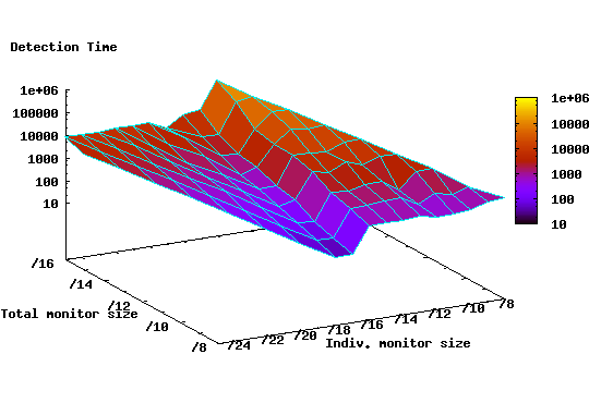Figure 11 shows the detection time for different size and number configurations under this scenario. Observe that for deployments with monitor unit sizes less than /16, the detection time is still significantly lower than equivalent deployments where random placement is used (cf. Figure 9). Specifically, the minimum detection time is 33 time ticks compared to 230 time ticks for random deployments. Moreover, notice that the minimum detection time is close to the minimum detection time (9 ticks) when perfect knowledge of the population density is available. This is an encouraging result since it shows that even with partial knowledge of the vulnerable population distribution, one still can significantly enhance the detection capability of the monitoring scheme.

7 Conclusion and Future Work

Monitoring unused IP space is an attractive approach for detecting security events such as active scanning worms. Recently, a number of research proposals have advocated the use of distributed network monitors to automatically detect worm outbreaks. Clearly, the effectiveness of such a monitoring system depends heavily on the monitors' ability to quickly detect new worm outbreaks. However, until now, a number of factors that have direct implications for the detection speed of distributed monitoring systems were left unanswered.

In this paper, we focus on the effect of three important factors, namely (i) the aggregate size of the monitored space, (ii) the number of monitors in the system, and (iii) the location of the monitors in the IP address space. Our results show that distributed monitors can have detection times that are 4 to 100 times faster when compared to single monitors of the same sizes. Additionally, we investigate whether information about the density of the vulnerable population can be used to improve detection speed, and our results show that even given partial knowledge the impact on detection is substantial; for some deployments the detection time is seven times as fast compared to analogous monitor configurations where monitors are deployed randomly in the IP space. While precise knowledge about the vulnerable population distribution is probably unattainable, particularly at a global scale, we contend that establishing incremental knowledge of population density by major service providers is not intractable.

As part of our future work, we plan to conduct a more in-depth evaluation of the locality and stationary of the vulnerable population, and how that impacts monitoring practices. Moreover, we plan to explore other challenges associated with distributed monitoring, particularly its resilience to monitor failures and misinformation, efficient strategies for information sharing, and appropriate communication protocols to support this task.

Acknowledgments

This work is supported in part by National Science Foundation grant SCI-0334108. We thank DShield for graciously providing access to their IDS logs, and Vinod Yegneswaran for his assistance with the data. We also thank CAIDA for making the Witty dataset available. Lastly, we extend our gratitude to the reviewers for their insightful comments and feedback.

Bibliography

1

Computing Research Association.
CRA conference on grand research challenges in Information Security and Assurance, November 2003.

2

Michael Bailey, Evan Cooke, Farnam Jahanian, Jose Nazario, and David Watson.
Internet motion sensor: A distributed blackhole monitoring system.
In Proceedings of the ISOC Network and Distributed System Security Symposium (NDSS), 2005.

3

The CAIDA Dataset on the Witty Worm - March 19-24, 2004, Colleen Shannon and David Moore, https://www.caida.org/passive/witty/. Support for the Witty Worm dataset and the UCSD Network Telescope are provided by Cisco Systems, Limelight Networks, DHS, NSF, CAIDA, DARPA, Digital Envoy, and CAIDA Members.

4

Z. Chen, L. Gao, and K. Kwiat.
Modeling the Spread of Active Worms.
In Proceedings of IEEE INFOCOMM, volume 3, pages 1890 - 1900, 2003.

5

Evan Cooke, Michael Bailey, Z. Morley Mao, David Watson, Farnam Jahanian, and Danny McPherson.
Toward Understanding Distributed Blackhole Placement.
In Proceedings of ACM Workshop on Rapid Malcode WORM04, pages 54-64, October 2004.

6

Symantec Corporation.W32.Blaster.Worm.
https://securityresponse.symantec.com/avcenter/venc/data/w32.blaster.worm.html,
August 2003.

7

Distributed Intrusion Detection System (DShield).
https://www.dshield.org/

8

"eEye Digital Security".
Code Red-II Worm Analysis.
https://www.eeye.com/html/Research/Advisories/ AL20010804.html.

9

"eEye Digital Security". Code Red Worm.
https://www.eeye.com/html/Research/Advisories/ AL20010717.html.

10

G. Gu, M. Sharif, X. Qin, D. Dagon, W. Lee, and G. Riley.
Worm Detection, Early Warning and Response Based on Local Victim Information.
In Proceedings of Annual Computer Security Applications Conference, December 2004.

11

H.W. Hethcote.
The Mathematics of Infectious Diseases.
In SIAM Reviews, Vol. 42 No. 4, 2000.

12

Andrew Mackie, Jenssen Roculan, Ryan Russel, and Mario Van Velzen.
Nimda Worm Analysis.
https://aris.securityfocus.com/alerts/nimda/010919-Analysis-Nimda.pdf
2001

13

D. Moore, G. Voelker, and S. Savage.
Inferring Internet Denial of Service Activity.
In Proceedings of $10^{th}$ USENIX Security Symposium, August 2001.

14

David Moore.
Network Telescopes: Observing Small or Distant Security Events.
In $11^{th}$ USENIX Security Symposium, Invited Talk, August 2002.

15

David Moore, Collen Shannon, and Jeffry Brown.
Code-Red: A case study on the spread and victims of an Internet worm.
In Proceedings of Internet Measurement Workshop, pages 273-284, November 2002.

16

The North America Networks Operators' Group (NANOG) mailing list.
Available at https://www.nanog.org/mailinglist.html.

17

Routeviews- University of Oregon.
https://www.routeviews.org/

18

Colleen Shannon and David Moore.
The Spread of the Witty Worm.
IEEE Security and Privacy Magazine, 2(4):46-50, July 2004.

19

S. Staniford, V. Paxson, and N. Weaver.
How to 0wn the internet in your spare time.
In Proceedings of the $11^{th}$ USENIX Security Symposium, August 2002.

20

Stuart Staniford, David Moore, Vern Paxson, and Nick Weaver.
The Top Speed of Flash Worms.
In Proceedings of the ACM Workshop on Rapid Malcode (WORM), pages 33-42, October 2004.

21

J. Wu, S. Vanagala, L. Gao L., and K. Kwiat.
An Effective Architecture and Algorithm for Detecting Worms with Various Scan Techniques.
In Proceedings of the ISOC Network and Distributed System Security Symposium (NDSS), 2004.

22

V. Yegneswaran, P. Barford, and J. Somesh.
Global Intrusion Detection in the DOMINO Overlay System.
In Proceedings of the ISOC Network and Distributed Systems Security Symposium (NDSS), 2004.

23

C. Zou, L. Gao, W. Gong, and D. Towsley.
Monitoring and Early Warning of Internet Worms.
In Proceedings of ACM Conference on Computer and Communications Security (CCS), pages 190-199, October 2003.

24

Cliff Zou, D. Towsley, Weibo Gong, and Songlin Cai.
Routing Worm: A Fast, Selective Attack Worm based on IP Address Information.
UMass ECE Technical Report TR-03-CSE-06, November 2003.

25

C. Zu, W. Gong, and D. Towsley.
Code Red Worm Propagation Modeling and Analysis.
In Proceedings of ACM Conference on Computer and Communication Security (CCS), pages 138-147, 2002.

26

C. Zu, W. Gong, and D. Towsley.
Worm Propagation Modeling and Analysis under Dynamic Quarantine Defense.
In Proceedings of the ACM Workshop on Rapid Malcode (WORM), pages 51-60, 2003.

Footnotes

... scanners.¹

We also detect and filter out vertical scanning sessions (scans from a single source targeting multiple ports on the same destination host), so only horizontal scanning activity (analogous to worms behavior) is used in our analysis.

...) ²

The PDF of the Log-Normal distribution is given by:
$P(x)=\frac{e^{-(\ln x- m)^2/2s^2}}{s \sqrt{2 \pi} x}$

... malicious³

In practice a more sophisticated anomaly detection scheme need be applied to classify true malicious scans from benign hits.

... sizes ⁴

The choice of unit sizes is somewhat arbitrary, but the main goal is to cover a wide range of possibilities in order to depict the interaction between number and size of monitors.

Security '05 Technical Program Security '05 Home USENIX home