Security '05 Paper [Security '05 Technical Program]

Vulnerabilities of Passive Internet Threat Monitors

Yoichi Shinoda
Japan Advanced Institute of Science and Technology
Ko Ikai
National Police Agency, Japan
Motomu Itoh
Japan Computer Emergency Response Team Coordination Center (JPCERT/CC)

Abstract

Passive Internet monitoring is a powerful tool for measuring and characterizing interesting network activity like worms or distributed denial of service attacks. By employing statistical analysis on the captured network traffic, Internet threat monitors gain valuable insight into the nature of Internet threats. In the past, these monitors have been successfully used not only to detect DoS attacks or worm outbreaks but also to monitor worm propagation trends and other malicious activities on the Internet. Today, passive Internet threat monitors are widely recognized as an important technology for detecting and understanding anomalies on the Internet in a macroscopic way.

Unfortunately, monitors that publish their results on the Internet provide a feedback loop that can be used by adversaries to deduce a monitor's sensor locations. Knowledge of a monitor's sensor location can severely reduce its functionality as the captured data may have been tampered with and can no longer be trusted. This paper describes algorithms for detecting which address spaces an Internet threat monitor listens to and presents empirical evidences that they are successful in locating the sensor positions of monitors deployed on the Internet. We also present solutions to make passive Internet threat monitors "harder to detect".

1 Introduction

Back in the good old days, observing traffic at addresses that never generated packets themselves was rare and was assumed to be solely due to poorly engineered software or misconfiguration. Nowadays, hosts connected to the Internet constantly receive probe or attack packets, whether they are silent or not. It is an unfortunate fact that most of these packets are generated and sent by entities with malicious intentions in mind.

Observing these packets from a single vantage point provides only limited information on the cause behind these background activities, if any at all. Capturing packets from multiple monitoring points and interpreting them collectively provides a more comprehensive view of nefarious network activity. The idea of monitoring background traffic dates back to CAIDA's network telescope in 2000 [1]. CAIDA uses a huge, routed, but very sparsely populated address block. Another approach has been taken by DShield [2] which is a distributed and collaborative system that collects firewall logs from participating system administrators.

Both CAIDA and DShield were successfully used not only to infer DoS attacks on remote hosts [3], but also to monitor the activity of existing malware [4], and to detect outbreaks of new malware. The success of these systems has resulted in the deployment of many similar monitoring facilities around the World. Some of these new monitor deployments feature a large contiguous address space like CAIDA's telescope and others are similar to DShield's architecture in the sense that they listen on addresses widely distributed over the Internet. In this paper, we will collectively refer to these systems as passive Internet threat monitors. Today, Internet threat monitors are considered as the primary method to observe and understand Internet background traffic in a macroscopic fashion.

However, we have noticed that most passive threat monitors that periodically publish monitor results are vulnerable to active attacks aimed at detecting the addresses of listening devices, or sensors. In our study, we successfully identified the sensor locations for several monitors in a surprisingly short time when certain conditions are met. For some monitors, we were able to locate majority of deployed sensors.

The operation of Internet threat monitors relies on a single fundamental assumption that sensors are observing only non-biased background traffic. If sensor addresses were known to adversaries then the sensors may be selectively fed with arbitrary packets, leading to tainted monitor results that can invalidate any analysis based on them. Similarly, sensors may be evaded, in which case sensors are again, effectively fed with biased inputs. Furthermore, volunteers who participate in deploying their own sensors face the danger of becoming DoS victims which might lower their motivation to contribute to the monitoring effort. Because passive threat monitors are an important mechanism for getting a macroscopic picture background activities on the Internet, we must recognize and study the vulnerability of these monitors to protect them.

The rest of the paper is organized as follows. In Section 2, we provide a brief introduction to passive threat monitors, followed by a simple example of an actual detection session in Section 3. In section 4, vulnerabilities of passive threat monitors are closely examined by designing detection algorithms. We discuss properties of feedback loops provided by threat monitors, develop detection algorithms that exploit these properties, and determine other important parameters that collectively characterize detection activities. Finally, in Section 6, we show how to protect passive threat monitors from these threats. While some ideas and thoughts presented are immediately applicable but their effectiveness is somewhat limited, others are intended for open discussion among researchers interested in protecting threat monitors against detection activities.

Although we focus on sensor detectability of distributed threat monitors, it is straightforward to extend our discussion to large telescope-type monitors also.

2 Passive Internet Threat Monitors

2.1 Threat Monitor Internals

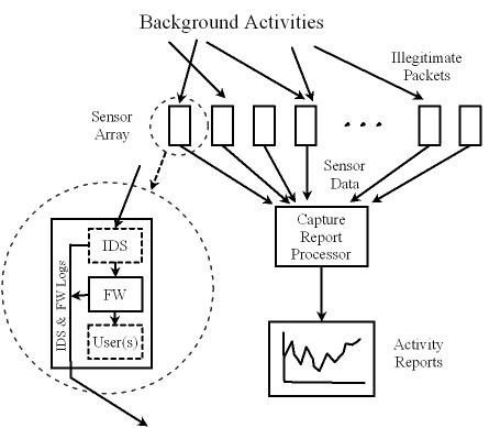
Figure 1 shows a typical passive Internet threat monitor. It has an array of sensors listening to packets arriving at a set of IP addresses, capturing all traffic sent to these addresses. Logs of capture events are sent to capture report processor where these events are gathered, stored, processed and published as background activity monitor reports. Some sensors monitor network traffic for large address spaces, while others capture only packets sent to their own addresses.

A passive sensor often functions like a firewall that is configured to record and drop all packets. The sensor may also be equipped with an IDS of some kind to explicitly capture known attacks. A sensor may be a dedicated "silent" device that never generates packets by itself, or it may have users behind it in which case its firewall must be configured to pass legitimate packets in both directions.

Figure 1: Structure of a Typical Internet Threat Monitor

2.2 Characterizing Threat Monitors

To properly characterize passive threat monitors, we need to look at their two main aspects: the properties of their sensors and the reports they provide. In the following, we provide a brief discussion of both so that readers get a better understanding of the basic principles behind Internet threat monitors.

2.2.1 Properties of Sensors

Sensor Aperture: A Sensor may monitor a single address, or multiple addresses simultaneously. We call the size of the address space a sensor is listening to its aperture. Examples of sensors with extremely large aperture are systems monitoring routed but empty or sparsely populated address space, such as the CAIDA's telescope [1] and the IUCC/IDC Internet Telescope [5]. CAIDA's telescope is claimed to monitor a /8 space, and IUCC/IDC Internet Telescope is claimed to monitor a /16 space.
Sensor Disposition: Some systems use multiple sensors that are distributed across the Internet address space, while others just use a single sensor. Extreme examples of a highly distributed sensor are DShield [2] and the Internet Storm Center [4]. They explain their system as monitoring over 500,000 addresses spanning over 50 different countries around the World [6].
Sensor Mobility: Sensors may be listening to fixed addresses or dynamically assigned addresses, depending on how they are deployed. Large, telescope type sensors with extremely large aperture such as /8 are likely to be listening on fixed addresses, while small aperture sensors, especially those hooked up to DSL providers are very likely to be listening to dynamically changing addresses.
Sensor Intelligence: Some systems deploy firewall type sensors that capture questionable packets without deep inspection, while others deploy intrusion detection systems that are capable of classifying what kind of attacks are being made based on deep inspection of captured packets.
There are some sensors that respond to certain network packets making them not quite "passive" to capture payloads that all-drop firewall type sensors cannot. [7,8].
Sensor Data Authenticity: Some systems use sensors prepared, deployed and operated by institutions, while others rely on volunteer reports from the general public.

We see no fundamental difference between traditional, so called "telescope" threat monitors and "distributed sensor" threat monitors as they all listen to background traffic. In this paper, we focus on detecting sensors of distributed threat monitors, but it is straightforward to extend our discussion to large telescope monitors.

2.2.2 Report Types

All reports are generated from a complete database of captured events, but exhibit different properties based on their presentation. There are essentially two types of presentation styles: the data can be displayed as "graph" or in "table" format.

Port Table Table type reports tend to provide accurate information about events captured over a range of ports. Figure 2 shows the first few lines from a hypothetical report table that gives packet counts for observed port/protocol pairs.

% cat port-report-table-sample # port proto count 8 ICMP 394 135 TCP 11837 445 TCP 11172 137 UDP 582 139 TCP 576 :

Figure 2: An Example of Table Type Report

Time-Series Graph The graph type reports result from visualizing an internal database, and tend to provide less information because they summarize events. The graphs we will be focusing on are the ones that have depict explicit time-series, that is, the graph represents changes in numbers of events captured over time. Table type reports also have time-series property if they are provided periodically, but graphs tend to be updated more frequently than tables.

Figure 3 shows an hypothetical time-series graph report. It contains a time-series of the packets received per hour for three ports, during a week long period starting January 12th.

We examine other report properties in detail in Section 4.2.

Figure 3: An Example of Time Series Graph Feedback, showing only three most captured events.

2.3 Existing Threat Monitors

In addition to threat monitors already mentioned, there are many similar monitors deployed around the World. For example, SWITCH [9] operate telescope type monitors.

Examples of distributed sensor monitors are the monitor run by the National Police Agency of Japan [10], ISDAS (Internet Scan Data Acquisition System) run by JPCERT/CC [11] and WCLSCAN [12] which is unique in that it uses sophisticated statistical algorithms to estimate background activity trends. The IPA (Information-Technology Promotion Agency, Japan) is also known to operate two versions of undocumented threat monitor called TALOT (Trends, Access, Logging, Observation, Tool) and TALOT2.

University of Michigan is operating the Internet Motion Sensor, with multiple differently sized wide aperture sensors [13,14]. Telecom-ISAC Japan is also known to operate an undocumented and unnamed threat monitor that also combines several different sensor placement strategies. PlanetLab[15] has also announced a plan to build their own monitor based on distributed wide aperture sensors.

Building and deploying a threat monitor is not a cumbersome task for anyone with some unoccupied address space in hand. For example, the Team Cymru Darknet Project provides a detailed step by step guideline for building a monitor [16].

3 The Problem

3.1 A Simple Example

To demonstrate that our concerns are realistic, we show that we can identify the addresses of real network monitor sensors. Let us consider one example; we omit some details about the discovered monitors to not compromise their integrity. The monitor we were investigating provides a graph of the top five packet types that gets updated once an hour. Without any prior knowledge, properties of this monitor were studied using publicly available materials such as symposium proceedings, workshop handouts and web sites. It became clear that there is a high likelihood that at least one of its sensors was located in one of four small address blocks.

We examined the graph to determine if we could find a way to make obvious changes to it by sending appropriately typed packets to the suspected addresses ranges. The graph showed the top 5 packet types with a granularity of only one week, so introducing a new entry into the graph would require a substantial number of packets. It was something that we didn't want to do. Instead, the existing entries were examined, and one of the UDP ports was chosen as a target, because of its constant low-profile curve. So, we sent a batch of empty UDP packets using the previously chosen port number to each address in the candidate blocks, covering one block every hour.

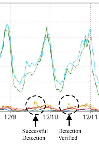
Figure 4: The graph shows the feedback from the simple marking session. The target curve is shown in dark yellow, and spikes produced by sending UDP packets are emphasized in dotted circles.

Four hours later, we examined the report graph from this monitor on the web, part of which is shown in Figure 4, and found a spike of the expected height in the curve; labeled "Successful Detection." Because we knew the time at which we sent packets to each address block, it was obvious which of the four blocks contained the sensor. For verification purposes, the same procedure was repeated on the suspect block next day, and produced another spike in the feedback graph, labeled "Block is Verified" in the Figure.

3.2 The Impact

In this paper, we are investigating vulnerabilities of threat monitors that break either implicit or explicit assumptions that are fundamental to a monitors' functionality. The biggest assumption that all monitors rely on is that they are observing non-biased background traffic.

However, as shown in the simple example presented in the previous section, sensor address detection is not totally impossible. Our study shows that proper analysis of the target system leads to detection in surprisingly short time.

In the following, we examine possible consequences after sensor addresses have become known.

Sensors may be fed with arbitrary packets.
Sensors may be fed selectively with arbitrary packets. The result is that captured events no longer represent general background activity, effectively disabling the target monitor.
Sensors may become DoS victims.
Furthermore, sensors may be subject of DoS attacks, possibly disabling victim sensors and associated networks. The risk of suffering a DoS attack or actually having been attacked may result in volunteers removing their sensors from the distributed monitors reducing their effectiveness.
Sensors may be evaded.
Malicious activity may evade sensors. Again, capture results no longer represent general background activity.

It is important to realize that sensor attackers or evaders do not require a complete list of sensor addresses. The list may be incomplete, or it may include address ranges instead of addresses. The sensor revocation mentioned above could be triggered by a single address or address range in the list.

It is equally important to recognize that these vulnerabilities are not limited to systems that make results publicly available. There are commercial services and private consortium which run similar threat monitors and provide their clients or members with monitor results with certain precision. We all know that information released to outside organizations is very likely to be propagated among unlimited number of parties whether or not the information is protected under some "soft" protection. Therefore, the threat is the "Clear and Present Danger" for anybody who runs similar services.

4 Detection Methods

To understand the vulnerabilities of threat monitors, we first investigate possible ways of detecting them.

4.1 The Basic Cycle

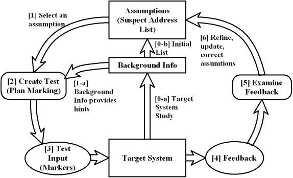
The scheme that we have used for sensor detection is basically a variation of the classic black-box estimation procedure, as shown in Figure 5.

Figure 5: The Monitor Detection Cycle

In Figure 5, a target system is at the bottom, and what we call an assumption pool is at the top. This pool holds address lists or address ranges that we believe might host sensors. The goal of the detection procedure is to refine assumptions in this pool as much as possible. An outline of the procedure is described below.

The target system is studied prior to the actual detection procedure (0-a). Background information about the target system's characteristics are collected using publicly available information such as conference proceedings, workshop handouts, talk videos and web pages.
Properties of feedback information (reports) from the target systems are also of interest in this phase, and is discussed in Section 4.2. Characteristics of an operating institution, including relationships with other institutions and personal relationships between key people sometimes allow us to derive valuable information about sensor deployment.
As a result of this process, an initial set of address lists or address ranges may be determined and stored in the assumption pool (0-b). Background information may also be filled with parameters that affect the detection cycle. This includes a wide range of information, from available physical resources to various policies.
The actual detection cycle starts by selecting an address list or address range from the pool. The list or range may be divided into smaller lists or ranges if necessary.
We design a set of tests to refine the selected assumption - usually narrowing down its range. To distinguish this process from the traditional " scanning", we call running these tests "marking".
Various background information, especially feedback properties of the target system, are used in this process (1-a). We call the packets used in marking activities "markers". The main focus in the design process is the marking algorithm deployed, which is discussed in Section 4.3. Details of designing the marking activity are discussed in Section 4.4.
We run the marking process against the target system by sending markers to addresses in the suspected address list or range.
We capture the feedback from the target system.
The feedback is examined to identify results of successful marking.
Based on these results, the assumption is refined, corrected, or updated. Afterwards, a new cycle begins with a newly selected assumption.

4.2 Feedback Properties

The feedback properties that a target monitor provides influence the marking process in many ways. In the following, we examine the major properties of typical feedbacks. The most obvious property is the feedback type, either a table or a graph, which we already described in Section 2.2.2.

4.2.1 Timing Related Properties

For feedback in the form of a time series, timing related properties play an important role when designing marking activity.

Accumulation Window

The accumulation window can be described as the duration between two consecutive counter resets. For example, a feedback that resets its counter of captured events every hour has a accumulation window of one hour.

The accumulation window property affects the marking process in several different ways;

An attempt to introduce changes must happen within the accumulation window period. In other words, the accumulation window determines the maximum duration of a unit marking activity.
The smaller the accumulation window the more address blocks can be marked in a given time frame.
A smaller accumulation window requires less markers to introduce changes.

Time Resolution

Time resolution is the minimum unit of time that can be observed in a feedback. The time resolution provides a guide line for determining the duration of a single marking activity. That is, a single marking activity should be designed to fit loosely into multiples of the time resolution for the target system. We can not be completely accurate as we need to be able to absorb clock skew between target and marking systems.

Feedback Delay

Delay is the time between a capture event and next feedback update. For example, a feedback that is updated hourly has a maximum delay of one hour, while another feedback that is updated daily has a maximum delay of one day. The delay determines the minimum duration between different marking phases that is necessary to avoid dependency between them.

Most feedbacks have identical time resolution, accumulation window and delay property, but not always. For example, there is a system which provides a weekly batch of 7 daily reports, in which case the accumulation window is one day while the maximum delay is 7 days.

Retention Time

The retention time of a feedback is the maximum duration that a event is held in the feedback. For a graph, the width of the graph is the retention time for the feedback. All events older than the graph's retention time are pushed out to the left.

Figure 6 illustrates the relationship between different timing properties using a hypothetical feedback that updates every 2 days, and provides accumulated packet counts for a particular day every 6 hours. As shown in this figure, this feedback has a time resolution of 6 hours, a accumulation window of 1 day, a maximum feedback delay of 2 days. In addition, the retention time for this graph is 3 days. The duration of some possible marking activities are also shown in this figure. Note that a marking activity can span multiple resolution units, but cannot span two accumulation windows.

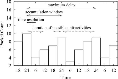Figure 6: Timing Properties of A Hypothetical Feedback

4.2.2 Other Feedback Properties

In addition to the timing related properties, there is a group of properties that mainly rule how capture events are presented in feedbacks. These properties also play an important role when designing marking activity.

Type Sensitivity: Type sensitivity refers to the sensitivity of a feedback to certain types of packets. If a feedback shows significant changes in its response to an appropriate amount of packets of the same type, then the feedback is sensitive to that type.
Dynamic Range: The dynamic range of a feedback, which is the difference between smallest and largest numbers in the feedback, presents another important factor in a marking design, in conjunction with the level sensitivity property described next.
Counter Resolution / Level Sensitivity: The counter resolution of a feedback is the minimal number of packets required to make an identifiable change in the feedback. For example, a feedback table that includes information for a single event has a resolution of 1 packet, while the feedback in a graph that is 100 dots high with a maximum scale (dynamic range) of 1,000 packets has a resolution of 10 packets.
We use the term "sensitivity" also to describe the "level of sensitivity". In the above example, the former feedback is more sensitive than the latter feedback. Some systems use logarithmic scale for their feedbacks, and as a result, they are sensitive to small spikes even if the dynamic range of the feedback is very large.
The unit of measurement also vary from system to system, and affects the level sensitivity of the feedback. Some use accumulated packet counts directly, in which case the sensitivity can be calculated easily. Others use mathematically derived values such as average packet counts per sensor and packet counts per 100 sensors. In the latter case, number of sensors in the monitor must be known to calculate the sensitivity. This figure may be obtained from the background information for the monitor, or may be estimated by comparing the feedback with feedbacks from other monitors that use plain packet counts.
Cut-off and Capping: Some systems drop events that are considered non-significant. Some systems drop events that are too significant, so events with less significance are more visible. A common case of cut-off is a feedback in the form of "Top-N" events. In this type of feedback, the top N event groups are selected, usually based on their accumulated event count over a predetermined period of time such as an hour, a day or a week. A feedback with the top-N property is usually very hard to exploit, because it often requires a large number of events to make significant changes such as visible spikes or an introduction of a new event group. However, there is a chance of exploiting such feedback, when the feedback exhibits certain properties, such as frequently changing members with low event counts, or if there is a event group with a period of inactivity. An introduction of a new event group is also possible, by "pre-charge" activity that is intended to accumulate event counts.

4.3 Marking Algorithms

An algorithm used for a particular marking is often depends on the feedback properties. It is sometimes necessary to modify or combine basic marking algorithms to exploit a particular feedback, or to derive more efficient marking algorithm. In the following, we present some examples of possible marking algorithms.

4.3.1 Address-Encoded-Port Marking

A system providing a table of port activities may become a target of an address-encoded-port marking. In this method, an address is marked with a marker that has its destination port number derived from encoding part of the address bits. After the marking, port numbers which were successfully marked are recovered from the feedback, which are in turn combined with other address bits to derive refined addresses.

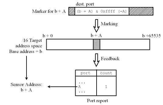
Consider the case in Figure 7. In this example, we mark a /16 address block with base address b that is hosting a sensor at b + A. The destination port of the marker for address b + n is set to the 16 lower bits of the address b + n (which is equivalent to n). For the sensor address b + A, a marker with destination port set to A is sent, which in turn appear as captured event on port A in the port activity report. This feedback is combined with the base address b to form the complete address of the sensor, which is b + A.

Figure 7: An Address-Encoded-Port Marking Example

Although the address-encoded-port marking can only be deployed against table type feedbacks, it is considered extremely efficent, because it can deliver multiple complete or partial addresses from a single marking activity.

However, not all of the 16-bit port space is available in practice; there are ports which are frequently found in real background activity. Some of these ports, especially those that are used by vulnerable, usually receive a large number of events. Other ports may also receive some background traffic due to back scatter and stray or wandering packets.

To increase the accuracy of our method even in the presence of background traffic for some ports, it is possible to determine the usable port space in advance. This can be achieved by looking at previous port-reports from the target system. The accuracy of this method can also be improved by incorporating redundant marking in which multiple makers of the same type are sent to the same address to mask the existence of busy ports.

Redundant marking also helps in dealing with packet losses. For example, we can mark a particular address with four different markers, each using a destination port number that is encoded with 2-bits of redundancy identifier and 14-bits of address information. In this case, we examine the feedback for occurrences of these encoded ports.

4.3.2 Time Series Marking

Time series marking can be used when the feedback is in the form of a time series property. It is used in conjunction with other marking algorithms such as the uniform intensity marking described next. In time series marking, each sub-block is marked within the time resolution window of the feedback so that results from marking can be reverse back to the corresponding sub-block.

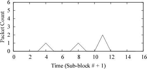
4.3.3 Uniform Intensity Marking

In uniform-intensity marking, all addresses are marked with the same intensity. For example, let's assume that we are marking a /16 address block that is known to contain several sensors. We divide the original block into 16 smaller /20 sub-blocks. Then we mark each of these sub-blocks using time-series marking, one sub-block per time unit, marking each address with a single marker.

Figure 8: An Example of Uniform-Intensity Marking Feedback

Figure 8 shows an ideal (no packet loss, and all other conditions being good) feedback graph from the marking described above. In this figure, the vertical axis represents the packet count and the horizontal axis represents time. We see that there is a spike of height one at time 4, which means that there is one sensor in sub-block #3, since the packet count at time 4 is accumulated between time 3 and time 4, when sub-block #3 was being marked. Similarly, there is a spike of height one at time 8 and height two at time 11, meaning there is one sensor in sub-block #7 and two sensors in sub-block #10.

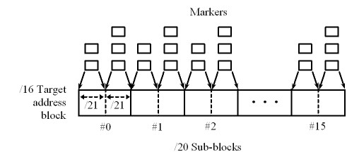
4.3.4 Radix-Intensity Marking

In radix-intensity marking, selected address bits are translated into marking intensity, i.e., the number of packets for each address. Let us consider the example used in the uniform-intensity section above. We execute the same marking procedure, but mark the first /21 block within a sub-block with 2 markers, and the second /21 block with 3 markers (Figure 9). Table 1 shows the possible location of sensors within a sub-block, and how they are reflected in the feedback intensity.

Figure 9: An Example of Radix-Intensity Marking

	Sensor Location (Block #)
	first	second	third	Feedback
Count	sensor	sensor	sensor	Intensity
0	-	-	-	0
1	0	-	-	2
	1	-	-	3
2	0	0	-	4
	0	1	-	5
	1	1	-	6
3	0	0	0	6
	0	0	1	7
	0	1	1	8
	1	1	1	9

Table 1: Single Bit (2 for 0 and 3 for 1) Radix-Intensity Feedback for up to 3 sensors in a sub-block.

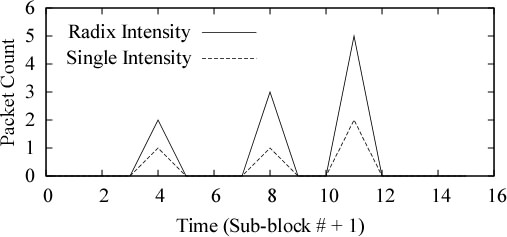
Figure 10: An Example of Radix-Intensity Marking Feedback

For this example, we further assume that there are no more than two sensors in each sub-block. Figure 10 shows the ideal feedback from this marking with solid lines. The feedback from the uniform-intensity marking is also drawn for comparison in dotted lines. Looking at the solid line, we notice a spike with height 2 at time 4 meaning that there is one sensor in the first half of sub-block #4. There is also a spike with height 3 at time 8 meaning that there is one sensor in the second half of sub-block #7. Another spike spike with height 5 can be seen at time 11 meaning that there are two sensors, one in the first and another in the second half of sub-block #10.

Notice that with uniform-intensity marking, the feedback would have derived only the numbers of sensors in each sub-block, while radix-intensity marking was able to also derive information about the positions of these sensors within each sub-block. For this example, the radix-intensity marking derived an extra bit of address information.

In radix-intensity marking, the assignment of intensity to address bit patterns has to be designed carefully to minimize the ambiguity during feedback translation. The above example used intensities 2 and 3 for a single bit. As shown in Table 1, this assignment allows unique decoding of up to two sensors in a single sub-block, and with a single exception, it allows unique decoding of up to three sensors in a single sub-block (there is an ambiguity for feedback intensity value of 6 which decodes into two cases).

In practice, code assignment has to consider the effect of packet loss, so the assignment becomes more complicated. Another drawback of the radix-intensity marking is that aggressive encoding introduces unusually large spikes in the feedback. The number of address bits that are encoded as intensity should be kept relatively small so that the marking activity can retain its stealthiness.

4.3.5 Radix-Port Marking

When several ports are available for marking, a port pair can be assigned to toggle an address bit off or on (0/1). Multiple pairs can be used to encode multiple address bits, but we need to be careful that traces of multiple event groups do not interfere with each other.

4.3.6 Delayed Development Marking

This is yet another marking algorithm, that can be combined with the other more fundamental marking algorithms.

This method is especially useful when the feedback is a graph that displays "Top-N" activity. In time-series marking on this type of feedback, we have to be sure that results of successful hits are noticeable in the feedback by using the appropriate marking intensity for each address. However, since Top-N graphs show only frequently captured events, it is often necessary to use high intensities to make significant changes.

Delayed development marking solves this problem by deploying two separate phases of marking which we call "exposure" phase and "development" phase. These terms were taken from the classical silver-oxide photography in which a hidden image accumulated on a medium by exposure to light is later developed to produce a visible image.

Our algorithm use markers instead of light. In the exposure phase, marking is done with minimal intensity markers, leaving hidden traces in the feedback. The intensity for this phase is the minimal sensitivity level of the feedback, and the duration of the phase is determined from the retention time of the feedback. After the exposure phase but within the retention time of the feedback, development marking is done with high intensity markers. This will introduce a new event group into the feedback, revealing all hidden traces. Of course, it is necessary that the development marking hits the sensor for successful development. Thus, it is desirable to have several known addresses for successful marking using this algorithm.

A variation of the algorithm exploits the inactivity period of existing or recurring top-N event groups. In this case, the explicit development phase is not necessary, since the natural background activity will effectively develop the hidden traces. An example of this exploit is given in section 5.2.

4.3.7 Combining Algorithms

As noted already earlier, it is possible to create new algorithms by combining or varying the algorithms we have presented. For example, an algorithm that spans different feedback types is also possible.

4.4 Designing A Marking Activity

An actual marking activity can be characterized by several parameters. Some of these parameters are interrelated, so the process of designing a marking activity cannot be fixed. In the following, we describe the typical process of designing a marking activity.

Target Range
First, we need to decide on the range, or the block of addresses that we want to mark. The initial range may be determined from social engineering, reasonable guesses or a combination of both. For example, sensors for a monitor run by a national CERT are likely to be placed in the address assigned to that nation. Without any information, we essentially have to start with the full /0 address space, except for the bogons, i.e. the unroutable addresses ranges. Later markings can use the results from preceding markings.

Marking Algorithm
The marking algorithm is basically determined by the properties of the selected feedback. If the feedback is in table form, then the address-encoded-port marking would be a good candidate. If the feedback is in the form of a graph, time-series marking with one of the intensity-based algorithms would be a decent candidate. Variations of selected algorithms to exploit the space that the feedback provides are also considered here.

Marker Design
The marker packet is designed next.

Marker type
Protocol, source and destination port number are determined from the requirements of the selected algorithm and the feedback's type sensitivity.

Source address
The source IP address of marking packets may be spoofed because we do not require a reply to them. The only information we require is the data from feedback reports which can obtained independently of the marking packets. However, spoofed source addresses may affect the stealthiness of the marking activity. If someone running the target monitor were to examine the source addresses of packets they capture, addresses belonging to Bogon (un-routable) address space would certainly draw attention. So, randomly generated source addresses should be avoided. A list of non-Bogon addresses can be generated by taking a snapshot of BGP routing table from a core Internet router. Another easy way is to use the addresses of actual attackers obtained by running a passive packet monitor.

Payload
The presence of a payload is also considered here based on the sensor type. While most firewall type sensors are sensitive to small packets including TCP handshaking segments and payload-less UDP datagrams, most IDS type sensors require a payload that the IDS is sensitive to.

Intensity
The intensity of a marking specifies how many markers are sent to a single address, and is usually determined from the resolution and the noise level of a feedback. The selected marking algorithm may impose additional constraints, and we may also need to take the stealthiness into account.

Bandwidth
The bandwidth parameter depends on limiting factors imposed by the availability of physical resources, capacity of bottleneck routers, or our stealthiness requirements. If a botnet of an appropriate size can be utilized, the bandwidth is not a limiting parameter. Nevertheless, we assume that we have some concrete bandwidth figure here.

Velocity
The velocity of a marking is the speed with which marker packets can be generated. The bandwidth cap on the velocity can be calculated from the bandwidth parameter above and the marker size, but the actual velocity is also limited by the CPU speed of the host generating the markers. For example, with a naive generator based on libnet [17], a 350 MHz Intel Celeron can generate only 100 small markers per second, while the same software on a 2.4 GHz Intel Pentium 4 can generate packets of the same size 15 times faster. Nevertheless, whichever smaller becomes the actual velocity.

Address Range Subdivision
The number of addresses that can be marked per unit time is calculated from the velocity and the intensity. This figure together with the feedback's timing properties discussed in Section 4.2 determines the number of addresses that can be marked in a time unit. This number also determines how a target range is sub-divided into smaller sub-blocks.

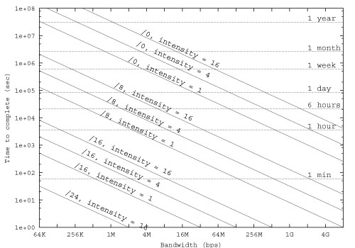
At this point, if a derived sub-block size is too big or to small, or not appropriate by some other reason, then parameters already determined above should be adjusted. As readers might have noted, there is a inter-relationships among bandwidth, intensity, sub-block size and marking duration. Figure 11 is a chart that shows this dependency for 64-byte markers, in a form of bandwidth against duration for various sized address blocks and selected intensity. In reality, these inter-relating parameters are ought to be tweaked around using the chart like this one.

Figure 11: Bandwidth v.s. Time for Various Sized Blocks and Intensities for 64-byte Markers

Marking Order
The order in which we mark blocks or addresses within a block may increase or decrease the likelihood of our marking activity being detected. One example would be the presence of an advanced IDS that does spatial and longitudinal analysis of captured events. For this reason, we may want to scramble the order in which we send the markers in some way or other.

4.5 Gathering Additional Information

There are several supplemental procedures that can be used to gather additional information before or in between series of marking activities.

ICMP-Based Recon: Some systems explicitly state that their sensors respond to ICMP requests to attract and capture packets from adversaries who check if a target host is alive prior to an actual attack. This feature can be used to select a set of candidates from a target region prior to the actual marking process.
Sensor Fingerprinting: There are threat monitors, especially those prepared and deployed by large organizations that use uniform hardware and software platforms for their sensors. In this case, once the first sensor has been detected, it can be fingerprinted to help with identifying additional sensors of the same type.
For the purpose of detecting sensors of threat monitors, ICMP is the only method we can use. However, our study shows that we can fingerprint the sensors that respond to ICMP requests to some extent by characterizing their responses to various ICMP requests, such as Echo Requests, Timestamp Requests, Mask Requests, or Information Requests.
Topological inference: For sensors to be useful, it is necessary that they are deployed in fashion that gives them access to as much traffic as possible. In particular, it is often undesirable to deploy sensors behind firewalls or small network segments. Therefore, it seems likely that sensors deployed within an intranet are not placed deeply in the topology. So, for address blocks assigned to intranets, we can use tools like traceroute to study their internal topology, and then carry out our marking activity can against those address blocks closer to the ingress point of the intranet. Note that address blocks assigned to intranets can be identified through the use of whois and similar tools. The fact that surprisingly many hosts respond to ICMP Mask Requests can also be used to build a topology map of a particular intranet. It is ironic that features which facilitate administrating Internet hosts provide us with an improved way to compromise another class of systems intended for Internet management.
FQDN filtering: At some stage in the detection process, candidate addresses may be converted into FQDNs via DNS reverse lookups. We can then examine their names and drop those from the list that contain words that indicate some common purpose, such as "www", "mail" or "ns". This filter is particularly useful for address ranges that cover intranets. In our experience, this kind of filtering actually cut down the number of addresses in the candidate list from 64 to only 2.

For some of these algorithms, it is necessary to use a non-spoofed source address because they require bidirectional interaction with hosts and routers in or near the target region. The drawback of using non-spoofed addresses is that traffic from them may be easier to detect and could alert monitor operators to the fact that their sensors are under attack.

5 Case Studies

We have successfully determined the addresses of several sensors belonging to multiple threat monitors. In this process, we employed actual marking using live networks and simulated environments but also mathematical simulations. In this section, we present some significant cases that can be discussed without compromising the security of the vulnerable monitors.

5.1 System A

System A corresponds to the threat monitor described in the introductory example in Section 3.1. As described earlier, in our initial study of the system, we were able to derive four small address blocks that we suspected to host sensors. We used time-series uniform-intensity marking on each block and disovered that there was actually one sensor in one of the blocks.

This system provides a feedback report in the form of a port table in addition to the graph type feedback used in the first cycle. The second cycle was run using the address-encoded-port marking on the block determined in the first cycle, using 4 redundantly encoded markers per address. To remain undetected, we scrambled the markers so that there was no obvious relationship between bit patterns of sensor addresses and port numbers. From the feedback, the complete address of the sensor was successfully decoded.

During the feedback delay of the second cycle, another set of methods was tested on this block. First, the ICMP-recon on addresses on this block was run. The address block was scanned with ICMP echo request, connection request (TCP-SYN) on 22/tcp and 1433/tcp. Addresses that respond to ICMP echo request but did not respond to connection requests were kept in the list, which finally held 227 addresses. Since the original block was /22 (1024 addresses), the ICMP-recon has cut down the size of the list to one-fifth. Then, the list was put through FQDN-filter. Since this block was assigned to a intranet, almost all addresses in the list were resolved into names that resembles some kind of a particular function, except two addresses. These two addresses were marked with time-series uniform-intensity marking on ICMP echo request, and revealed a complete sensor address, which indeed matched with the results from the second cycle.

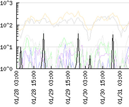
5.2 System B

This is an imaginary case, but can be applied to many existing threat monitors. The "Dabber Worms" hitting 9898/tcp is very well known to have explicit period of activity and inactivity, as shown in Figure 12. The active period always last for few hours at fixed time of the day, followed by inactive period that last until next active period. Events captured during the active period is likely to be in the range of 1-10 per sensor, depending on the monitor. On the other hand, virtually no events are captured during the inactive period, except for occasional spikes that goes as high as one event per sensor.

Figure 12: A Typical Dabber Worm Event Profile in Solid Black Lines (Vertical Axis is total events captured expressed in log scale). The period of inactivity provides a good space for marking in a Top-N type graph.

As readers might have noticed already, the activity profile and intensity figures of the Dabber Worm profile provides graphs containing this profile to be exploited during the period of inactivity. The simplest example would be a time-series uniform-intensity marking using destination 9898/tcp. The marking intensity depends on how feedback intensity is presented, but because of the activity profile of the Dabber Worm, this event group should stay or recur in the graph (delayed development marking with autonomous development phase).

5.3 System C

This is another existing system, that publishes daily accumulated port reports that covers entire port range. This type of feedback is a target for the address-encoded-port marking. However, the problem (or the strength) of this system is that it deploys numerous number of sensors, and as a result, the port report table is very noisy. Most ports are occupied, and clean ports are hard to predict.

However, the port report provided by this system includes not only total event counts, but also numbers of different sources and targets for each port, as shown in Figure 13.

port total events # of src # of tgt 0 17630 1367 533 1 188 37 27 2 123 20 21 ... 65535 47 9 5

Figure 13: A Hypothetical Port Report From System C

Examination of these figures reveals that there are strong statistical trends in these reports. Take ratio of number of targets and number of sources (#targets/#sources, abbreviated as TSR here after) for example.

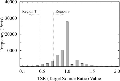
Figure 14: Target/Source (TSR) Value Distribution Example

Figure 14 shows a distribution of TSR values, calculated from the actual port report from this system, on a particular day in December 2004. Each bar represents occurrences of values smaller than the corresponding horizontal label (inclusive), and larger than the next smaller horizontal label (exclusive). Clean ports (no reports, no sources, no destinations) are counted as having TSR=1.0 for convenience. From this graph, we see the obvious strong bell shaped distribution with TSR=1.0 at the center.

Because we can always mark with spoofed source addresses, we can manipulate the TSR value for a particular port to be smaller than it actually would, by marking the port with different source addresses. Now, let us define two regions in the distribution graph, Region S and Region T as in Figure 14. Here, Region S is where ports to be marked reside, and Region T is where ports marked should move into. That is, if we can move ports that were otherwise in Region S into Region T by reasonable number of markers with different source addresses, and if we can detect these movements, then we have a variation of the address-encoded-port marking.

One way to implement this marking is to use the yesterday's port report to identify ports that could have been moved if they were marked, and use these ports as address encoding space for today's marking activity. This sounds very naive, but if counts on ports tend to change gradually from day to day, it should work.

Below is the outline of the algorithm, using standard statistical operations to determine threshold values for Region S and T.

From yesterday's port table, drop ports with EC (event count) > 100. These are ports with incredibly large event counts that affect the statistical operations of this algorithm. Since we will never manipulate these ports, it is safe to drop them first.
We do the same thing with some more precision. Compute average and standard deviation of remaining reports, avg (EC) and stddev (EC) respectively, and drop those ports with EC >= avg (EC) + stddev (EC). These ports are unlikely to move.
Compute TSR value for all remaining ports, and also compute their average avg (TSR) and stddev (TSR).
Let STHRESH, the threshold value for Region S to avg (TSR) - stddev (TSR).
Let TTHRESH, the threshold value for Region T to STHRESH - 0.5 × stddev (TSR). Leaving little space between Region S and T avoids ports in Region S that should not move from wondering into Region T.
From remaining ports, select ports with TSR > STHRESH.
For each of the selected port, add nmarker to number of sources, add 1 to number of targets, and calculate a new TSR. This simulates "what if marked with nmarker different sources" situation.
If the new TSR <= TTHRESH, then add the port to the encoding space. The port "could have been moved".
Sort the encoding space in ascending order, using EC as a sort key. This is because lower count ports are easier to manipulate.
Trim the encoding space so that the size of the space is 2ⁿ. At this point, we have a encoding space for n-bit.
Run an actual address-encoded-port marking using the encoding space, and obtain the feedback.
Look for ports with TSR <= TTHRESH in the feedback.

We can confirm the validity of this whole idea by running a simulation of this algorithm using port reports from the target system. An encoding space is generated from the port report of the first day, then all ports in the encoding space are marked artificially in the port report of the second day. The result of the artificial marking can then be evaluated as follows.

False Positive: The original TSR of a port was already in Region T without marking. The algorithm will still detect this port as a successful marking, so this is a false positive case.
Successful Marking (Hit): The original TSR was in Region S, and the artificial marking moved this port into Region T. This is a successful marking.
False Negative: The original TSR was in Region S, and the artificial marking could not move this port into Region T.

Note that this type of simulation yields a more precise evaluation of the algorithm than running an actual marking. As results from the actual marking are affected by the disposition of actual sensors in the target address region, we would not know the correct number of actual sensors. The simulation derives the probability of successful markings, under the assumption that all addresses in the target region host sensors.

We simulated this algorithm against 30 pairs of actual port reports from 31 consecutive days in December 2004, with encoding space size set to 16,384 (14-bit). Also, nmarker, number of markers, was set to stddev(EC), unless stddev(EC) is greater than 16, in which case nmarker was set to 16. Table 2 only shows results for the first week, but other dates came up with similar numbers. The last column shows result of 4-way majority marking, in which hit is counted when at least 3 out of 4 markers satisfy the hit condition.

Date

mean TSP

sthresh

tthresh

nmarker

Hits (%)

FP (%)

FN (%)

3o4 (%)

12/02

0.965

0.738

0.625

88.8

0.1

11.1

93.5

12/03

0.848

0.638

0.533

94.8

2.1

3.1

98.6

12/04

0.881

0.654

0.540

88.2

0.5

11.3

93.2

12/05

0.838

0.553

0.410

87.2

12.3

0.5

92.1

12/06

0.835

0.648

0.554

95.3

0.3

4.4

99.3

12/07

0.842

0.660

0.570

95.0

0.1

4.9

98.7

12/08

0.851

0.674

0.586

94.7

0.4

4.9

98.5

Table 2: Result of Simulated Marking for First Week of Dec. 2004.

As shown in this table, the algorithm does perform well, despite the fact that it is quite naive. In fact, the 4-way redundant marking with 'at least 3 out of 4' majority condition achieves almost perfect results, even though it reduces the available port-space to one quarter of the original size. More sophisticated ways of trend analysis that derive better port space may further improve the performance, especially in the non-redundant case.

For some day-pairs, the number of markers, or intensity, can be much smaller, some times as small as 8 markers without sacrificing the performance. However, the table shows mechanically computed value, which is based on standard deviation of event counts, which is for stealthiness. The intensity seems unrelated to any of the statistical values we have used in our example algorithm, so there must be something that we have missed here. Nevertheless, with intensity of at most 16 markers, this algorithm is capable of revealing at least 12-bits from this monitor per day.

6 Protecting Threat Monitors

As mentioned earlier, threat monitors are inherently vulnerable to marking activities. Possible approaches to protect these monitors is discussed in this section, starting with assessment of the Leak. By knowing the how much information the monitor is leaking, we can infer the time-to-live for sensors and the monitor, which in turn can be used to take correct measures.

6.1 Assessing the Leak

The first step of the monitor protection is to assess how much information is leaking per unit time. An important guideline for the assessment is that we should not totally rely on figures derived by some explicit procedure in mind.

A hypothetical example would show this. Assume that there is a hypothetical monitor that publishes a completely unpopulated table type port report every hour. Let's assume that there are 1K sensors in this monitor. A botnet with 20K hosts each shooting address-encoded-port type markers at 30 marker/sec will produce a complete list of /16 blocks where sensors are placed in the very first hour. Then during the second hour, each /16 block is marked with address-encoded-port markers each using 64 port (6 bits), producing a complete list of /22 blocks. This process is repeated, and at the end of 4th hour, complete list of full 32-bit addresses for all 1K sensors will be produced.

The process may become shorter, depending on number of blocks produced by each phase. If 1K sensor addresses are actually 128 wide aperture sensors each monitoring a /28 space, then the each phase will produce maximum of 128 blocks, which means that we can use 512 ports (11-bit worth) for second and third phases, and the complete list would be available after the 3rd hour.

As shown here, the same marking activity behaves differently under different conditions. So the procedurally derived assessment results should only be used as a reference.

6.2 Possible Protections

Provide Less Information
An obvious way to fight against marking activities is to decrease the amount of information the system is giving out, prolonging the time-to-live. Manipulating feedback properties studied in section 4.2 will provide a good starting point. For example, longer accumulation window, longer feedback delay, less sensitivity, and larger cut-off threshold all works for this purpose. However, there are several points that we have to be aware of.

Frequency and level of detail of published reports usually reflect a system's basic operation policy. For example, some system expect large-scale distributed (manual) inspection by report viewers so that new malicious activities can be captured at its very early stage. Such system obviously requires frequent and detailed reports to be published, and decreasing the amount of information given may interfere with this policy. Therefore, there is a trade off between the degree of protection by this method and the fundamental policy of the system.
Even if we decrease the amount of information, we still have a leak. So, the amount of information the system is giving out should be decided with theoretical considerations, and should never be decided by some simplistic thoughts.

Giving out background information that leads to acquisition of vital system parameters or valuable additional information should be kept minimum. This includes system overview statements that are open to public, such as those in system's home pages, proceedings and meeting handouts. Some system is required to disclose its internals to some extent by its nature. The information disclosed should still be examined carefully even if this is the case.

Throttle the Information
There seem to be some standard remediation techniques that are being used to provide privacy in data mining that could be applied here. It would be helpful to study the privacy of database queries and relate it to the problem presented in this paper.

Introducing Explicit Noise
Because of the stealthiness requirement, most marking activities would try to exploit small changes in feedbacks. Adding small noise to captured events would disturb capturing the small changes. The noise can be artificially generated, but authors believe that this is something we should not do. One possible way is to introduce explicit variance into level sensitivity into sensors. For example, sensors can be divided into two groups, in which one group operates at full sensitivity, and another group operates at a reduced sensitivity, generating low level noise like events. Theoretically speaking, this method can be understood as introducing another dimension that markings have to consider. In this sense, levels of sensitivity should be different across all sensors, rather than limiting them to only two levels.

The similar effect can be introduced by inter-monitor collaboration, in which noise is generated from monitor results from other monitor systems, using them as sources for legitimate noise.

Disturbing Mark-Examine-Update Cycle
Another obvious way is to disturb the mark-examine-update cycle in figure 5 so that list of addresses will not get refined, or at least slowing down the cycle. One way to implement this strategy is to incorporate explicit sensor mobility.

Things to consider here are:

Degree of mobility required to disturb the cycle must be studied. Assuming that marking activities do not use address bit scrambling (for stealthiness purposes), it is obvious that changing addresses within a limited small address space does little harm to the cycle, because the cycle only have to discard the last part of its activity. Conversely, moving among much larger blocks would invalidate the marking result at its early stage, impacting all results thereafter.
Current threat monitors that use different set of almost identical sensors and almost identical post-processing provide different reports. Our guess is that with the number of sensors these systems are using, location of sensors affects the monitor result quite a bit. So, degree of how sensor mobility affects monitor results must be studied, together with further investigation for reasoning of multiple threat monitors giving different results. A study using variations in sensor aperture and placement [18] gives answers to some of these questions.

Intentionally discarding part of captured events in random or other fashion also disturbs the mark-examine-update cycle. From the view point of consistency of monitor results, this method is better than explicit mobility. However, it must be noted that discarding events will deteriorate the effective sensitivity of the monitor.

Marking Detection
Another obvious and powerful, but hard to implement way is to detect marking activities and discard associated capture events. This is extremely difficult, because well designed marking is expected to give least correlations among markers and thus nearly indistinguishable from real background activities.

However, there is a fundamental difference between marking activities and real background activities; events generated by marking activities are basically local and transient by nature. It may be possible to design a marking activity that implicitly covers multiple addresses and that persist over time, but only at the sacrifice of marking speed. We are now looking at several ways to handle transient events. Statistical approach may work in some cases, especially for those activities that introduce strong statistical anomalies, and we have already gathered some positive result from the statistical filtering approach.

Correlations among different monitors may be used to detect marking activities, but again, difference among feedbacks from different monitors must be studied in depth first. We are also not certain if this method would be capable of detecting small transient changes. In any case, we believe that studies on advanced IDS would provide another good starting point.

Sensor Scale and Placement
Consider an imaginary case in which 2¹⁶ sensors are placed uniformly over the /16 blocks (one sensor per /16 block) for example. This arrangement forces address-encoded-port marking to be applied sequentially until half of sensors are detected. Although the marking still derives complete sensor addresses at constant rate during this period, the arrangement effectively slows down the most efficient marking method. Increasing number of sensors that are carefully placed provide a certain level of protection, and worth studying its property.

The carefully planned distributed sensor placement may also benefit the marking detection efforts, by revealing patterns of the transient events that sweeps across address blocks.

Small Cautions
In section 4.5, we have pointed out several additional methods to gather useful information. Most of these methods can be disabled by paying small attentions.

Give FQDNs to sensors deployed in intranets to prevent FQDN-based filtering. Names that resembles common functionality, or names that dissolves into other hosts in the same subnet are better choices.
For ICMP-echo-responding sensors, consider answering to some other packets they capture, to prevent them from detected as silent host that only answers to ICMP echo request.
Consider how sensors respond to various ICMP requests to prevent ICMP-based fingerprinting and topology inferencing.
For intranet-placed sensors, introduce some facility (hardware and/or software) such as TTL mangling, to make sensors look like they are deep inside a intranet to avoid topology inferencing based filtering.

7 Conclusion

Passive Internet threat monitors are an important tool for obtaining a macroscopic view of malicious activity on the Internet. In this paper, we showed that they are subject to detection attacks that can uncover the location of their sensors. We believe that we have found a new class of Internet threat, because it does not post a danger to the host systems themselves, but rather a danger to a meta-system that is intended to keep the host systems safe.

Although we believe that we have not fully defined the threat, we presented marking algorithms that work in practice. They were derived more or less empirically, so it is possible that there may be more efficient marking algorithms that we did not study. For example, methods for detecting remote capture devices has been studied in the context of remote sniffer detection, but none of these studies have correlated plain sniffers with threat monitors, and there may be techniques that can be applied in our context. To find insights that we may have missed, a more mathematical approach to the analysis of feedback properties may be necessary.

We presented some methods to protect against our markings algorithms, but some of these solutions are hard to implement, and others still need to be studied more carefully for their feasibility and effectiveness and most importantly, for their vulnerabilities. The goal of this paper is to bring attention of this problem to the research community and leverage people with various expertise, not limited to system and network security, to protect of this important technology. Continuing efforts to better understand and protect passive threat monitors are essential for the safety of the Internet.

Acknowledgments

We would like to present our sincere gratitude to multiple parties who admitted our marking activities on their networks and monitor systems during the early stage of this research. We must confess, that marking against them sometimes went well beyond the level of the back ground noise, and sometimes took a form of unexpectedly formatted packets. We would also like to acknowledge members of the WIDE Project, members of the Special Interest Group on Internet threat monitors (SIGMON) and the anonymous reviewers for thoughtful discussions and valuable comments. We must also note that the final version of this paper could not have been prepared without the sincere help of our paper shepherd Niels Provos.

References

[1]: CAIDA Telescope Analysis. https://www.caida.org/analysis/security/telescope/.
[2]: Distributed intrusion detection system. https://www.dshield.org/.
[3]: David Moore, Geoffrey M. Voelker, and Stefan Savage. Inferring Internet Denial-of-Service Activity. In 10th USENIX Security Symposium, August 2001.
[4]: SANS Internet Storm Center (ISC). https://isc.sans.org/.
[5]: The IUCC/IDC Internet Telescope. https://noc.ilan.net.il/research/telescope/.
[6]: About the Internet Storm Center (ISC). https://isc.sans.org/about.php.
[7]: Ruoming Pang, Vinod Yegneswaran, Paul Barford, Vern Paxson, and Larry Peterson. Characteristics of Internet Background Radiation. In Proceedings of the Internet Measurement Conference (IMC) 2004, October 2004.
[8]: Dug Song, Rob Malan, and Robert Stone. A Snapshot of Global Internet Worm Activity. Technical report, Arbor Networks Inc., 2001.
[9]: SWITCH Internet Background Noise (IBN). https://www.switch.ch/security/services/IBN/.
[10]: @police Internet Activities Monitored. https://www.cyberpolice.go.jp/english/obs_e.html.
[11]: JPCERT/CC Internet Scan Data Acquisition System (ISDAS). https://www.jpcert.or.jp/isdas/index-en.html.
[12]: Masaki Ishiguro. Internet Threat Detection System Using Bayesian Estimation. In Proceedings of The 16th Annual Computer Security Incident Handling Conference, June 2004.
[13]: Internet Motion Sensor. https://ims.eecs.umich.edu/.
[14]: Michael Bailey, Eval Cooke, Farnam Jahanian, Jose Nazario, and David Watson. Internet Motion Sensor: A Distributed Blackhole Monitoring System. In Proceedings of The 12th Anual Network and Distributed System Security Symposium. ISOC, February 2005.
[15]: PlanetLab. https://www.planet-lab.org/.
[16]: The Team Cymru Darknet Project. https://www.cymru.com/Darknet/.
[17]: libnet. https://libnet.sourceforge.net/.
[18]: Evan Cooke, Michael Bailey, Zhuoqing Morley Mao, David Watson, Farnam Jahanian, and Danny McPherson. Toward understanding distributed blackhole placement. In Proceedings of the 2004 ACM workshop on Rapid malcode, October 2004.

This paper was originally published in the Proceedings of the 14th USENIX Security Symposium,
July 31–August 5, 2005, Baltimore, MD
Last changed: 3 Aug. 2005 ch

Security '05 Technical Program

Security '05 Home

USENIX home