Eric Anderson, HP Labs <eric.anderson4@hp.com>
Storage tracing and analysis have a long history. Some of the earliest filesystem traces were captured in 1985 (26), and there has been intermittent tracing effort since then, summarized by Leung (20). Storage traces are analyzed to find properties that future systems should support or exploit, and as input to simulators and replay tools to explore system performance with real workloads.
One of the problems with trace analysis is that old traces inherently have to be scaled up to be used for evaluating newer storage systems because the underlying performance of the newer systems has increased. Therefore the community benefits from regularly capturing new traces from multiple sources, and, if possible, traces that put a heavy load on the storage system, reducing the need to scale the workload.
Most traces, since they are captured by academics, are captured in academic settings. This means that the workloads captured are somewhat comparable, but it also means that commercial workloads are under-represented. Microsoft is working to correct this by capturing commercial enterprise traces from their internal servers (23). Our work focuses on commercial NFS (6,28,25) workloads, in particular from a feature animation (movie) company, whose name remains blinded as part of the agreement to publish the traces. The most recent publically available NFS traces that we are aware of were collected in 2003 by Ellard (13). Our 2003 and 2007 traces (4) provide recent NFS traces for use by the community.
One difference between our traces and other ones is the data rates that we measured. Our 2003 client traces saw about 750 million operations per day. In comparison, the 2003 Ellard traces saw a peak of about 125 million NFS operations per day, and the 2007 Leung traces (20) saw a peak of 19 million CIFS operations/day. Our 2007 traces saw about 2.4 billion operations/day. This difference required us to develop and adopt new techniques to capture, convert, and analyze the traces.
Since our traces were captured in such a different environment than prior traces, we limit our comparisons to their workloads, and we do not attempt to make any claims about trends. We believe that unless we, as a community, collect traces from hundreds of different sites, we will not have sufficient data to make claims stronger than "this workload is different from other ones in these ways." In fact, we make limited comparison of the trends between our 2003 and 2007 traces for similar reasons. The underlying workload changed as the rendering techniques improved to generate higher quality output, the operating system generating the requests changed, the NFS protocol version changed, and the configuration of the clients changed because of standard technology trends.
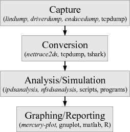
The process of understanding a workload involves four main steps, as shown in Figure 1. Our tools for these steps are shown in italics for each step, as well as some traditional tools. The first step is capturing the workload, usually as some type of trace. The second step is conversion, usually from some raw format into a format designed for analysis. The third step is analysis to reduce the huge amount of converted data to something manageable. Alternately, this step is a simulation or replay to explore some new system architecture. Finally the fourth step is to generate graphs or textual reports from the output of the analysis or simulation.
Our work has five main contributions:
We examine related work in Section 2. We describe our capture techniques in Section 3, followed by the conversion in Section 4. We describe our adopted and new analysis techniques in Section 5 and use them to analyze the workload in Section 6. Finally we conclude in Section 7.
The two closest pieces of related work are Ellard's NFS
study (13,12), and Leung's 2007 CIFS
study (20). These papers also summarize the earlier
decade of filesystem tracing, so we refer interested readers to those
papers. Ellard et al. captured NFS traces from a number of Digital
UNIX and NetApp servers on the Harvard campus, analyzed the traces and
presented new results looking at the sequentiality of the workload,
and comparing his results to earlier traces. Ellard made his tools
available, so we initially considered building on top of them, but
quickly discovered that our workload was so much more intense that his
tools would be insufficient, and so ended up building our own. We
later translated those tools and traces into DataSeries, and found our
version was about 100![]() faster on a four core machine and used
25
faster on a four core machine and used
25![]() less CPU time for analysis. Our 2003 traces were about
25
less CPU time for analysis. Our 2003 traces were about
25![]() more intense than Ellard's 2001 traces, and about 6
more intense than Ellard's 2001 traces, and about 6![]() more intense than Ellard's 2003 traces.
more intense than Ellard's 2003 traces.
Leung et al. traced a pair of NetApp servers on their campus.
Since the clients were entirely running the Windows operating system, his traces were of
CIFS data, and so he used the Wireshark tools (31) to
convert the traces. Leung's traces were of comparable intensity to
Ellard's traces, and they noted that they had some small packet drops
during high load as they just used tcpdump for capture. Leung identified and extensively analyzed
complicated sequentiality patterns.
Our 2007 traces were about 95![]() more intense than Leung's
traces, as they saw a peak of 19.1 million operations/day and we saw an
average of about 1.8 billion. This comparison is slightly misleading
as NFS tends to have more operations than CIFS because NFS is a
stateless protocol.
more intense than Leung's
traces, as they saw a peak of 19.1 million operations/day and we saw an
average of about 1.8 billion. This comparison is slightly misleading
as NFS tends to have more operations than CIFS because NFS is a
stateless protocol.
Tcpdump (30) is the tool that almost all researchers describe using to capture packet traces. We tried using tcpdump, but experienced massive packet loss using it in 2003, and so developed new techniques. For compatibility, we used the pcap file format, originally developed for tcpdump, for our raw captured data. When we captured our second set of traces in 2007, we needed to capture at even higher rates, and we used a specialized capture card. We wrote new capture software using techniques we had developed in 2003 to allow us to capture above 5Gb/s.
Tcpdump also includes limited support for conversion of NFS packets.
Wireshark (31) provides a graphical interface to packet
analysis, and the tshark variant provides conversion to text. We were
not aware of Wireshark at the time of our first capture, and we simply
adjusted our earlier tools when we did our 2007 tracing. We may
consider using the Wireshark converter in the future, provided we can
make it run much faster. Running tshark on a small 2 million packet
capture took about 45 seconds whereas our converter ran in about 5
seconds. Given conversion takes 2-3 days for a 5 day trace, we can not
afford conversion to slow down by a factor of 9![]() .
.
Some of the analysis techniques we use are derived from the database community, namely the work on cubes (16) and approximate quantiles (22). We considered using a standard SQL database for our storage and analysis, but abandoned that quickly because a database that can hold 100 billion rows is very expensive. We do use SQL databases for analysis and graphing once we have reduced the data size down to a few million rows using our tools.
The first stage in analyzing an NFS workload is capturing the data. There are three places that the workload could be captured: the client, the server, or the network. Capturing the workload on the clients is very parallel, but is difficult to configure and can interfere with the real workload. Capturing the workload on the server is straightforward if the server supports capture, but impacts the performance of the server. Capturing the workload on the network through port mirroring is almost as convenient as capture on the server, and given that most switches implement mirroring in hardware, has no impact on network or workload performance. Therefore, we have always chosen to capture the data through the use of port mirroring, if necessary, using multiple Ethernet ports for the mirrored packets.
The main challenge for raw packet capture is the underlying data rate. In order to parse NFS packets, we have to capture the complete packet. Because the capture host is not interacting with clients, it has no way to throttle incoming packets, so it needs to be able to capture at the full sustained rate or risk packet loss. To maximize flexibility, we want to write the data out to disk so that we can simplify the parsing and improve the error checking. This means that all of the incoming data eventually turns in to disk writes leading to the second challenge of maximizing effective disk space.
While the 1 second average rates may be low enough to fit onto the mirror ports, if the switch has insufficient buffering, packets can still be dropped. We discovered this problem on a switch that used per-port rather than per-card buffering. To eliminate the problem, we switched to 10Gbit mirror ports to reduce the need for switch-side buffering.
The capture host can also be overrun. At low data rates (900Mb/s, 70,000 packets/s), standard tcpdump on commodity hardware works fine. However, at high data rates (5Gb/s, 10^6 packets/s), traditional approaches are insufficient. Indeed, Leung (20) notes difficulties with packet loss using tcpdump on a 1 Gbit mirror port. We have developed three separate techniques for packet capture, all of which work better than tcpdump: lindump (user-kernel ring buffer), driverdump (in-kernel capture to files), and endacedump (hardware capture to memory).
The Linux kernel includes a memory-mapped, shared ring buffer for
packet capture. We modified the example lindump program to write out
pcap files (8), the standard output format from tcpdump, and
to be able to capture from more than one interface at the same time.
We wrote the output files to an in-memory filesystem using mmap to
reduce copies, and copied and compressed the files in parallel to
disk. Using an HP DL580G2, a current 4 socket server circa 2003,
lindump was able to capture about 3![]() the packets per second (pps) as
tcpdump and about 1.25
the packets per second (pps) as
tcpdump and about 1.25![]() the bandwidth. Combined with a somewhat
higher burst rate while the kernel and network card buffered data,
this approach was sufficient for mostly loss free captures at the animation
company, and was the technique we used for all of the 2003 set of
traces.
the bandwidth. Combined with a somewhat
higher burst rate while the kernel and network card buffered data,
this approach was sufficient for mostly loss free captures at the animation
company, and was the technique we used for all of the 2003 set of
traces.
Packets are captured into files in tmpfs, an in-memory filesystem, and then compressed
to maximize the effective disk space. If the capture host is mostly
idle, we compressed with gzip -9. As the backlog of pending
files increased, we reduced the compression algorithm to gzip
-6, then to gzip -1, and finally to nothing. In practice this
approach increased the effective disk size by 1.5-2.5![]() in our
experience as the data was somewhat compressible, but at higher input
rates we had to fall back to reduced compression.
in our
experience as the data was somewhat compressible, but at higher input
rates we had to fall back to reduced compression.
At another site, our 1Gbit lindump approach was insufficient because of packet bursts and limited buffering on the switch. Replacing the dual 1Gbit cards with a 10Gb/s card merely moved the bottleneck to the host and the packets were dropped on the NIC before they could be consumed by the kernel.
To fix this problem, we modified the network driver so that instead of passing packets up the network stack, it would just copy the packets in pcap format to a file, and immediately return the packet buffer to the NIC. A user space program prepared files for capture, and closed the files on completion. We called our solution driverdump since it performed all of the packet dumping in the driver.
Because driverdump avoids the kernel IP stack, it can
capture packets faster than the IP stack could drop them.
We increased the sustained packets per second over lindump by 2.25![]() to
676,000pps, and sustained bandwidth by 1.5
to
676,000pps, and sustained bandwidth by 1.5![]() to 170MiB/s (note 1 MiB/s =
to 170MiB/s (note 1 MiB/s = ![]() bytes/s). We could
handle short bursts up to 900,000 pps, and 215 MiB/s. This gave us
nearly lossless capture to memory at the second site. Since the files
were written into tmpfs, we re-used our technology for compressing and
copying the files out to disk.
bytes/s). We could
handle short bursts up to 900,000 pps, and 215 MiB/s. This gave us
nearly lossless capture to memory at the second site. Since the files
were written into tmpfs, we re-used our technology for compressing and
copying the files out to disk.
In 2007, we returned to the animation company to collect new traces on their faster NFS servers and 10Gb/s network. While an update of driverdump might have been sufficient, we decided to also try the Endace DAG 8.2X capture card (14). This card copies and timestamps packets from a 10Gb/s network directly into memory. As a result, it can capture minimal size packets at full bandwidth, and is intended for doing in-memory analysis of networks. Our challenge was to get the capture out to disk, which was not believed to be feasible by our technical contacts at Endace.
To solve this problem, we integrated our adaptive compression technique into a specialized capture program, and added the lzf (21) compression algorithm, that compresses at about 100MiB/s. We also upgraded our hardware to an HP DL585g2 with 4 dual-core 2.8Ghz Opterons, and 6 14 disk SCSI trays. Our compression techniques turned our 20TiB of disk space into 30TiB of effective disk space. We experienced a very small number of packet drops because our capture card limited a single stream to PCI-X bandwidth (8Gbps), and required partitioning into two streams to capture 10Gb/s. Newer cards capture 10Gb/s in a single stream.
Our capture techniques are directly applicable to anyone attempting to
capture data from a networked storage service such as NFS, CIFS, or
iSCSI. The techniques present a tradeoff. The simplest technique
(lindump), is a drop in replacement for using tcpdump for full packet
capture, and combined with our adaptive compression algorithm allows
capture at over twice the rate of native tcpdump and expands the
effective size of the disks by 1.5![]() . The intermediate
technique increases the capture rates by an additional factor of
2-3
. The intermediate
technique increases the capture rates by an additional factor of
2-3![]() , but requires modification of the in-kernel network
driver. Our most advanced techniques are capable of lossless
full-packet capture at 10Gb/s, but requires purchasing special capture
hardware. Both the lindump and driverdump code are available in our
source distribution (9). These tools and techniques
should eliminate problems of packet drops for capturing storage
traces. Further details and experiments with the first two techniques
can be found in (1).
, but requires modification of the in-kernel network
driver. Our most advanced techniques are capable of lossless
full-packet capture at 10Gb/s, but requires purchasing special capture
hardware. Both the lindump and driverdump code are available in our
source distribution (9). These tools and techniques
should eliminate problems of packet drops for capturing storage
traces. Further details and experiments with the first two techniques
can be found in (1).
Once the data is captured, the second problem is parsing and converting that data to a easily usable format. The raw packet format contains a large amount of unnecessary data, and would require repeated, expensive parsing to be used for NFS analysis. There are four main challenges in conversion: representation, storage, performance and anonymization. Data representation is the challenge of deciding the logical structure of the converted data. Storage format is the challenge of picking a suitable physical structure for the converted data. Conversion performance is the challenge of making the conversion run quickly, ideally faster than the capture stage. Trace anonymization is the challenge of hiding sensitive information present in the data and is necessary for being able to release traces.
One lesson we learned after conversion is that the converter's version number should be included in the trace. As with most programs, there can be bugs. Having the version number in the trace makes it easy to determine which flaws need to be handled. For systems such as subversion or git, we recommend the atomic check-in ID as a suitable version number.
A second lesson was preservation of data. An NFS parser will discard data both for space reasons and for anonymization. Keeping underlying information, such as per packet conversion in addition to per NFS-request conversion can enable cross checking between analysis. We caught an early bug in our converter that failed to record packet fragments by comparing the packet rates and the NFS rates.
One option for the representation is the format used in the Ellard (11) traces: one line per request or reply in a text file with field names to identify the different parameters in the RPC. This format is slow to parse, and works poorly for representing readdir, which has an arbitrary number of response fields. Therefore, we chose to use a more relational data structuring (7).
We have a primary data table with the common fields present in every request or reply, and an identifier for each RPC. We then have secondary tables that contain request-type specific information, such as a single table for RPC's that include attributes, and a single table for read and write information. We then join the common table to the other tables when we want to perform an analysis that uses information in both. Because of this structure, a single RPC request or reply will have a single entry in the common table. However, a request/reply pair will have zero (no entry in the read/write table unless the operation is a read/write) or more entries (multiple attribute entries for readdir+) in other tables.
The relational structuring improves flexibility, and avoids reading unnecessary data for analyses that only need a subset of the data. For example, an analysis only looking at operation latency can simply scan the common table.
Having decided to use a relational structuring for our data, we next
needed to decide how to physically store the data. Three
options were available to us: text, SQL, and DataSeries, our custom
binary format (2) for storing trace data.
Text is a traditional way of storing trace data, however, we were
concerned that a text representation would be too large and too slow.
Having later converted the Ellard traces to our format, we found that
the analysis distributed with the traces used 25![]() less CPU time when
the traces and analysis used DataSeries, and ran 100
less CPU time when
the traces and analysis used DataSeries, and ran 100![]() faster on a 4
core machine. This disparity confirmed our intuition that text is a
poor format for trace data.
faster on a 4
core machine. This disparity confirmed our intuition that text is a
poor format for trace data.
SQL databases support a relational structure. However, the lack of extensive compression means that our datasets would consume a huge amount of space. We also expected that many complex queries would not benefit from SQL and would require extracting the entire tables through the slow SQL connection.
Therefore, we selected DataSeries as an efficient and compact format for storing traces. It uses a relational data model, so there are rows of data, with each row comprised of the same typed columns. A column can be nullable, in which case there is a hidden boolean field for storing whether the value is null. Groups of rows are compressed as a unit. Prior to compression, various transforms are applied to reduce the size of the data. First, duplicate strings are collapsed down to a single string. Second, values are delta compressed relative to either the same value in the previous row or another value in the same row. For example, the packet time values are delta compressed, making them more compressible by a general purpose compression algorithm.
DataSeries is designed for efficient access. Values are packed so that once a group of rows is read in, an analysis can iterate over them simply by increasing a single counter, as with a C++ vector. Individual values are accessed by an offset from that counter and a C++ cast. Byte swapping is automatically performed if necessary. The offset is not fixed, so the same analysis can read different versions of the data, provided the meaning of the fields has not changed. Efficient access to subsets of the data is supported by an automatically generated index.
DataSeries is designed for generality. It supports versioning on the table types so that an analysis can properly interpret data that may have changed in meaning. It has special support for time fields so that analysis can convert to and from different raw formats.
DataSeries is designed for integrity. It has internal checksums on both the compressed and the uncompressed data to validate that the data has been processed appropriately. Additional details on the format, additional transforms, and comparisons to a wide variety of alternatives can be found in the technical report (10).
To perform the conversion in parallel, we divide the collected files into groups and process each group separately. We make two passes through the data. First, we parse the data and count the number of requests or replies. Second, we use those counts to determine the first record-id for each group, and convert the files. Since NFS parsing requires the request to parse the reply, we currently do not parse any request-reply pairs that cross a group boundary. Similarly, we do not do full TCP reconstruction, so for NFS over TCP, we parse multiple requests or replies if the first one starts at the beginning of the packet. These limitations are similar to earlier work, so we found them acceptable. We run the conversion locally on the 8-way tracing machine rather than a cluster because conversion runs faster than the 1Gbit LAN connection we had at the customer site (the tracing card does not act as a normal NIC). Conversion of a full data set (30TiB) takes about 3 days.
We do offline conversion from trace files, rather than online conversion, primarily for simplicity. However, a side benefit was that our converter could be paranoid and conservative, rather than have it try to recover from conversion problems, since we could fix the converter when it was mis-parsing or was too conservative. The next time we trace, we plan to do more on-the-fly conversion by converting early groups and deleting those trace files during capture so that we can capture longer traces.
In order to release the traces, we have to obscure private data such as filenames. There are three primary ways to map values in order to anonymize them:
We chose the last approach because it preserved the maximum flexibility, and allowed us to easily have discussions with the customer about unexpected issues such as writes to what should have been a read-only filesystem. Our encryption includes a self-check, so we can convert back to real filenames by decrypting all hexadecimal strings and keeping the ones that validate. We have also used the reversibility to verify for a colleague that they properly identified the '.' and '..' filenames.
We chose to encrypt entire filenames since the suffixes are specific to the animation process and are unlikely to be useful to people. This choice also simplified the discussions about publishing the traces. Since we can decrypt, we could in the future change this decision.
The remaining values were semi-random (IP addresses in the 10.* network, filehandles selected by the NFS servers), so we pass those values through unchanged. We decided that the filehandle content, which includes for our NFS servers the filesystem containing the file, could be useful for analysis. Filehandles could also be anonymized.
All jobs in the customers' cluster were being run as a common user, so we did not capture user identifiers. Since they are transitioning away from that model, future traces would include unchanged user identifiers and group identifiers. If there were public values in the traces, then we would have had to apply more sophisticated anonymization (27).
Analyzing the very large amount of data that we collected required us to adopt and develop new analysis techniques. The most important property that we aimed for was bounded memory, which meant that we needed to have streaming analysis. The second property that we wanted was efficiency, because without compute-time efficiency, we would not be able to analyze complete datasets. One of our lessons is that these techniques allowed us to handle the much larger datasets that we have collected.
Quantiles are better than simple statistics or histograms because they
do not accidentally combine separate measurements regardless of
distribution. Unfortunately, for our data, calculating exact quantiles
is impractical. For a single dataset, we collect multiple statistics
with a total of about 200 billion values. Storing all these values
would require ![]() 1.5TiB of memory, which makes it impractical
for us to calculate exact quantiles.
1.5TiB of memory, which makes it impractical
for us to calculate exact quantiles.
However, there is an algorithm from the database field for calculating
approximate quantiles in bounded
memory (22). A
q-quantile of a set of
n data elements is the element at position
![]() in the
sorted list of elements indexed from 1 to n. For approximate
quantiles, the user specifies two numbers
in the
sorted list of elements indexed from 1 to n. For approximate
quantiles, the user specifies two numbers ![]() , the maximum
error, and N, the maximum number of elements. Then when the program
calculates quantile q, it actually gets a quantile in the range
, the maximum
error, and N, the maximum number of elements. Then when the program
calculates quantile q, it actually gets a quantile in the range
![]() .
.
Provided that the total number of elements
is less than N, the bound is guaranteed. We have found that
usually the error is about 10![]() better than specified. For our
epsilon of 0.005 (sufficient to guarantee all percentiles are
distinct), instead of needing
better than specified. For our
epsilon of 0.005 (sufficient to guarantee all percentiles are
distinct), instead of needing ![]() 1.5TiB, we only need
1.5TiB, we only need
![]() 1.2MiB, an improvement of 10^6. This dramatic improvement
means we can run the analysis on one machine, and hence process
multiple sets in parallel. The performance cost of the algorithm is
about the same as sorting since the algorithm does similar sorting of
subsets and merging of subsets. Details on how the algorithm works
can be found in (22) or our software
distribution.
1.2MiB, an improvement of 10^6. This dramatic improvement
means we can run the analysis on one machine, and hence process
multiple sets in parallel. The performance cost of the algorithm is
about the same as sorting since the algorithm does similar sorting of
subsets and merging of subsets. Details on how the algorithm works
can be found in (22) or our software
distribution.
Calculating aggregate or roll-up statistics is an important part of
analyzing a workload. For example, consider the information in the
common NFS table: ![]() time, operation, client-id, and
server-id
time, operation, client-id, and
server-id![]() . We may want to calculate the total number of
operations performed by client 5, in which case we want to count the
number of rows that match
. We may want to calculate the total number of
operations performed by client 5, in which case we want to count the
number of rows that match ![]() *, *, 5, *
*, *, 5, *![]() .
.
The cube (16) is a generalization of the group-by
operations described above. Given a collection of rows, it calculates
the set of unique values for each column U(c), adds the special
value 'ANY' to the set, and then generates one row for each member of
the cross-product
![]() .
.
We implemented an efficient templated version of the cube operator for use in data analysis. We added three features to deal with memory usage. First, our cube can only include rows with actual values in it. This eliminates the large number of rows from the cross-product that match no rows in the base data. Second, we can further restrict which rows are generated. For example, we have a large number of client id's, and so we can avoid cubing over entries with both the client and operation specified to reduce the number of statistics calculated. Third, we added the ability to prune values out of the cube. For example, we can output cube values for earlier time values and remove them from the data structure once we reach later time values since we know the data is sorted by time.
The cube allows us to easily calculate a wide variety of summary statistics. We had previously manually implemented some of the summary statistics by doing explicit roll-ups for some of the aggregates described in the example. We discovered that the general implementation was actually more efficient than our manual one because it used a single hash table for all of the data rather than nested data structures, and because we tuned the hash function over the tuple of values to be calculated efficiently.
Our hash-table implementation (9) is a straightforward
chained-hashing implementation. In our experiments it is strictly
better in both performance and memory than the GNU C++ hash table. It
uses somewhat more memory than the Google sparse
hash (15), but performs almost as well as the
dense hash; it is strictly faster than the g++ STL hash. We added
three unusual features. First, it can calculate its memory usage,
allowing us to determine what needs to be optimized. Second, it can
partially reset iterators, which allows for safe mutating operations
on the hash table during iteration, such as deleting a subset of the
values. Third, it can return the underlying hash chains, allowing for
sorting the hash table without copying the values out. This operation destroys
the hash table, but the sort is usually done immediately before deleting the
table, and reduces memory usage by 2![]() .
.
Limiting memory usage for hash tables where the entries have unknown lifespan presents some challenges. Consider the sequentiality metric: so long as accesses are active to the file, we want to continue to update the run information. Once the file becomes inactive for long enough, we want to calculate summary statistics and remove the general statistics from memory. We could keep the values in an LRU data-structure. However if our analysis only needs a file id and last offset, then the forward and backwards pointers for LRU would double the memory usage. A clock-style algorithm would require regular full scans of the entire data structure.
We instead solve this problem by keeping two hash-maps, the recent and old hash-maps. Any time a value is accessed, it is moved to the recent hash-map if it is not already there. At intervals, the program will call the rotate(fn) operation which will apply fn to all of the (key,value) pairs in the old hash map, delete that map, assign the recent map to the old map and create a new recent map.
Therefore, if the analysis wants to guarantee any gap of up to 60 seconds will be considered part of the same run, it just needs to call rotate() every 60 seconds. Any value accessed in the last 60 seconds will remain present in the hash-map. We could reduce the memory overhead somewhat by keeping more than two hash-maps at the cost of additional lookups, but we have so far found that the rotating hash-map provides a good tradeoff between minimizing memory usage and maximizing performance. We believe that the LRU approach would be more effective if the size of the data stored in the hash map were larger, and the hash-map could compact itself so that scattered data entries do not consume excess space.
Once we have summarized the data from DataSeries using the techniques described above, we need to graph and subset the data. We combined SQL, Perl, and gnuplot into a tool we call mercury-plot. SQL enables sub-setting and combining data. For example if we have data on 60 second intervals, it is easy to calculate min/mean/max for 3600 second intervals, or with the cube to select out the subset of the data that we want to use. We use Perl to handle operations that the database can not handle. For example, in the cube, we represent the `ANY' value as null, but SQL requires a different syntax to select for null vs. a specific value. We hide this difference in the Perl functions. In practice, this allows us to write very simple commands such as plot quantile as x, value as y from nfs_hostinfo_cube where operation = 'read' and direction = 'send' to generate a portion of the graph. This tool allows us to deal with the millions of rows of output that can come from some of the analysis. To ease injection of data from the C++ DataSeries analysis, one lesson we learned is analysis should have a mode that generates SQL insert statements in addition to human readable output.
 |
| ||||||||||||||||||||||||||||||||||||||||||||||||||||||||||||||||||||||||||||||||||||||||||||||||||||||||||||
Analyzing very large traces can take a long time. While our custom binary format enables efficient analysis, and our analysis techniques are efficient, it can still take 4-8 hours to analyze a single set of the 2007 traces. In practice, we analyze the traces in parallel on a small cluster of four core 2.4GHz Opterons. Our analysis typically becomes bottle-necked on the file servers that serve up to 200MiB/s each once an analysis is running on more than 20 machines.
We collected data at two times: August 2003 - February 2004 (anim-2003), and January 2007 - October 2007 (anim-2007). We collected data using a variety of mirror ports within the company's network. The network design is straightforward: there is a redundant set of core routers, an optional mid-tier of switches to increase the effective port count of the core, and then a collection of edge switches that each cover one or two racks of rendering machines. Most of our traces were taken by mirroring links between rendering machines and the rest of the network. For each collected dataset, we would start the collection process, and let it run either until we ran out of disk space, or we had collected all the data we wanted. Each of these runs comprises a set. We have 21 sets from 2003, and 8 sets from 2007.
We selected a subset of the data to present, two datasets from 2003 and two from 2007. The sets were selected both because they are representative of the more intensive traces from both years, and to show some variety in the data. We identified clients as hosts that sent requests, servers as hosts that sent replies, and caches as hosts that acted as both clients and servers. Further information on each dataset can be found on the trace download page (4).
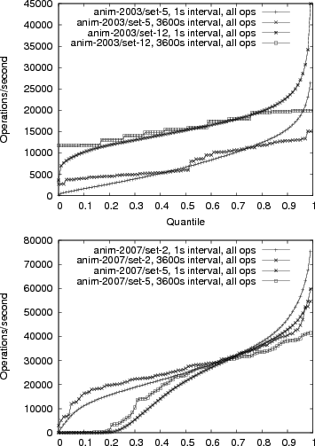
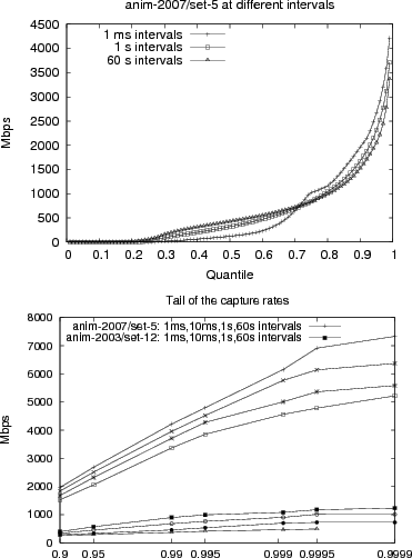
We start our analysis by looking at the performance of our capture tool. This validates our claims that we can capture packets at very high data rates. We examine the capture rate of the tool by calculating the megabits/s (Mbps) and kilo-packets/s (kpps) for 20 overlapping sub-intervals of a specified length. For example if our interval length is 60 seconds, then we will calculate the bandwidth for the interval 0s-60s, 3s-63s, 6s-66s, ... end-of-trace. We chose to calculate the bandwidth for overlapping intervals so that we would not incorrectly measure the peaks and valleys of cyclic patterns aligned to the interval length. We use the approximate quantile so we can summarize results with billions of underlying data points. For example, we have 11.6 billion measurements for anim-2007/set-0 at a 1ms interval length. This corresponds to the 6.7 days of that trace.
Figure 2(a) shows anim-2007/set-5 at different interval lengths. This graph shows the effectiveness of our tracing technology, as we have sustained intervals above 3Gb/s (358MiB/s), and 1ms intervals above 4Gb/s (476MiB/s). Indeed these traces show the requirement for high speed tracing, as 5-20% of the trace intervals have sustained intervals above 1Gbit, which is above the rate at which Leung (20) noted their tracing tool started to drop packets. The other sets from anim-2007 are somewhat less bursty, and the anim-2003 data shows much lower peaks because of our more limited tracing tools, and a wider variety of shapes, because we traced at more points in the network.
Figure 2(a) also emphasizes how bursty the traffic was during this trace. While 50% of the intervals were above 500Mbit/s for 60s intervals, only 30% of the intervals were above 500Mbit/s for 1ms intervals. This burstiness is expected given that general Ethernet and filesystem traffic have been shown to be self-similar (17,19), which implies the network traffic is also bursty. It does make it clear that we need to look at short time intervals in order to get an accurate view of the data.
Figure 2(b) shows the tail of the distributions for the capture rates for two of the trace sets. The relative similarity between the Mbps and kpps graphs is simply because packet size distributions are relatively constant. The traces show the remarkably high burstiness of the 2007 traces. While 90% of the 1ms intervals are below 2Gb/s, 0.1% are above 6Gb/s. We expect we would have seen slightly higher rates, but because of our configuration error for the 2007 capture tool, we could not capture above about 8Gb/s.
Examining the overall set of operations used by a workload provides insight into what operations need to be optimized to support the workload. Examining the distribution of rates for the workload tells us if the workload is bursty, and hence we need to handle a higher rate than would be implied by mean arrival rates, and if there are periods of idleness that could be exploited.
Table 1 provides an overview of all the operations that occurred in the four traces we are examining in more detail. It shows a number of substantial changes in the workload presented to the NFS subsystem. First, the read and write sizes have almost doubled from the anim-2003 to anim-2007 datasets. This trend is expected, because the company moved from NFSv2 to NFSv3 between the two tracing periods, and set the v3 read/write size to 16KiB. The company told us they set it to that size based on performance measurements of sequential I/O. The NFS version switch also accounts for the increase in access calls (new in v3), and readdirplus (also new in v3).
We also see that this workload is incredibly read-heavy. This is expected; the animation workload reads a very large number of textures, models, etc. to produce a relatively small output frame. However, we believe that our traces under-estimate the number of write operations. We discuss the write operation underestimation below. The abnormally low read size for set-12 occurred because that server was handling a large number of stale filehandle requests. The replies were therefore small and pulled down the bytes/operation. We see a lot more getattr operations in set-5 than set-12 because set-12 is a server behind several NFS-caches, whereas set-5 is the workload before the NFS-caches.
Table 2 and Figures 3(a,b) show how long averaging intervals can distort the load placed on the storage system. If we were to develop a storage system for the hourly loads reported in most papers, we would fail to support the substantially higher near peak (99%) loads seen in the data. It also hides periods of idleness that could be used for incremental scrubbing and data reorganization. We do not include the traditional graph of ops/s vs. time because our workload does not show a strong daily cycle. Animators submit large batches of jobs in the evening that keep the cluster busy until morning, and keep the cluster busy during the day submitting additional jobs. Since the jobs are very similar, we see no traditional diurnal pattern in the NFS load, although we do see the load go to zero by the end of the weekend.
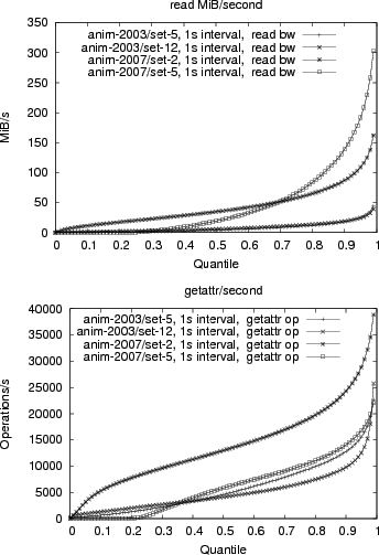
Figure 4 shows the read operation MiB/s and the getattr operations/s. It shows that relative to the amount of data being transferred, the number of getattrs has been reduced, likely a result of the transition from NFSv2 to NFSv3. The graph shows the payload data transferred, so it includes the offset and filehandle of the read request, and the size and data in the reply, but does not include IP headers or NFS RPC headers. It shows that the NFS system is driven heavily, but not excessively. The write operations/s graph (not shown for space reasons) implies that the write bandwidth has gotten more bursty, but has stayed roughly constant.
This result led us to further analyze the data. We were surprised
that write bandwidth did not increase, even though it is not
implausible, as the frame output size has not increased. We analyzed
the traces to look for missing operations in the sequence of
transaction ids, automatically inferring if the client is using a
big-endian or little-endian counter. The initial results looked quite
good: anim-2007/set-2 showed 99.7% of the operations were in sequence,
anim-2007/set-5 showed 98.4%, and counting the skips of 128 transactions
or less, we found only 0.21% and 0.50% respectively (the remaining
entries were duplicates or ones that we could not positively tell if
they were in sequence or a skip). However, when we looked one level
deeper at the operation that preceded a skip in the sequence, we found
that 95% of the skips followed a write operation for set-2, and 45%
for set-5. The skips in set-2 could increase the write workload by a
factor of 1.5![]() if all missing skips after writes are associated with
writes. We expected a fair number of skips for set-5 since we
experienced packet loss under load, but we did not expect it for
set-2.
if all missing skips after writes are associated with
writes. We expected a fair number of skips for set-5 since we
experienced packet loss under load, but we did not expect it for
set-2.
Further examination indicated that the problem came about because we followed the same parsing technique for TCP packets as was used in nfsdump2 (11). We started at the beginning of the packet and parsed all of the RPCs that we found that matched all required bits to be RPCs. Unfortunately, over TCP, two back to back writes will not align the second write RPC with the packet header, and we will miss subsequent operations until they re-align with the packet start. While the fraction of missing operations is small, they are biased toward writes requests and read replies. Since we had saved IP-level trace information as well as NFS-level, we could write an analysis that conservatively calculated the bytes of IP packets that were not associated with an NFS request or reply. Counting a direction of a connection if it transfers over 10^6 bytes, we found for anim-2007/set-2 that we can account for >90% of the bytes for 87% of the connections, and for anim-2007/set-5 that we can account for >90% of the bytes for >70% of the connections. The greater preponderance of missing bytes relative to missing operations reinforces our analysis above that the losses are due to non-aligned RPC's since we are missing very few operations, but many more bytes, and reads and writes have a high byte to operation ratio.
While this supports our lesson that retaining lower level information is valuable, this analysis also leads us to another one of our lessons: extensive validation of the conversion tool is important. Both validation through validation statistics, and through the use of a known workload that exercises the capture tools. An NFS replay tool (32) could be used to generate a workload, the replayed workload could be captured, and the capture could be compared to the original replayed workload. This comparison has been done to validate a block based replay tool (3), but has not been done to validate an NFS tracing tool, as the work has simply assumed tracing was correct. We believe a similar flaw is present in earlier traces (11) because the same parsing technique was used, although we do not know how much those traces were affected.
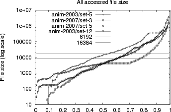
File sizes affect the potential internal fragmentation for a filesystem. They affect the maximum size of I/Os that can be executed, and they affect the potential sequentiality in a workload.
Figure 5 shows the size of files accessed in our traces. It shows that most files are small enough to be read in a single I/O: 40-80% of the files are smaller than 8KiB (NFSv2 read size) for the 2003 traces, and 70% of the files are smaller than 16KiB for the 2007 traces. While there are larger files in the traces, 99% of the files are smaller than 10MiB. The small file sizes present in this workload, and the preponderance of reads suggest that a flash file system (18) or MEMS file system (29) could support a substantial portion of the workload.
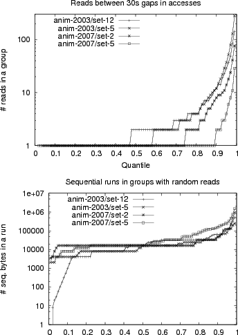
Sequentiality is one of the most important properties for storage systems because disks are much more efficient when handling sequential data accesses. Prior work has presented various methods for calculating sequentiality. Both Ellard (12) and Leung (20) split accesses into groups and calculate the sequentiality within the group. Ellard emulates opens and closes by looking for 30s groups in the access pattern. Ellard tolerates small gaps in the request stream as sequential, e.g. an I/O of 7KiB at offset 0 followed by an I/O of 8KiB at offset 8KiB would be considered sequential.
Ellard also reorders I/Os to deal with client-side reordering. In particular, Ellard looks forward a constant amount from the request time to find I/Os that could make the access pattern more sequential. This constant was determined empirically. Leung treats the first I/O after an open as sequential, essentially assuming that the server will prefetch the first few bytes in the file or that the file is contiguous with the directory entry as with immediate files (24). For NFS, the server may not see a lookup before a read, depending on whether the client has used readdir+ to get the filehandle instead of a lookup.
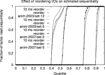
We determine sequentiality by reordering within temporally overlapping requests. Given two I/Os, A and B, if the request-reply intervals overlap, then we are willing to reorder the requests to improve estimated sequentiality. We believe this is a better model because the NFS server could reorder those I/Os. In practice, Figure 7 shows that for our traces this reordering makes little difference. Allowing reordering an additional 10ms beyond the reply of I/O A slightly increases the sequentiality, but generally not much more than just for overlapping requests.
We also decide on whether the first I/O is sequential or random based on additional I/Os. If the second I/O (after any reordering) is sequential to the first one, than the first I/O is sequential, otherwise it is random. If there is only one I/O to a particular file, then we consider the I/O to be random since the NFS server would have to reposition to that file to start the read.
Given our small file sizes, it turns out that most accesses count as random because they read the entire file in a single I/O. We can see this in Figure 6(a), which shows the number of reads in a group. Most groups are single I/O groups (70-90% in the 2007 traces). We see about twice as many I/Os in the 2003 traces, because the I/Os in the 2003 traces are only 8KiB, rather than 16KiB.
Sequential runs within a random group are more interesting. Figure 6(b) shows the number of bytes accessed in sequential runs within a random group. We can see that if we start accessing a file at random, most (50-80%) of the time we will do single or double I/O accesses (8-32KiB). However we also get some extended runs within a random group, although 99% of the runs are less than 1MiB.
 |
We have described three improved techniques for packet capture on networks. The easily adopted technique should allow anyone capturing NFS, CIFS, or iSCSI traffic from moderate performance storage systems (<= 1Gbit) to capture traffic with no losses. The most advanced technique allows lossless capture for 5-10Gbit storage systems, which is at the high end of most file storage systems. The primary lesson from this part of the work is that lossless 1Gbit packet capture is straightforward and up to 10Gbit is possible with an investment in development time or specialized hardware.
We have provided guidelines for conversion for future practitioners: parallelizing the conversion, retaining lower-level information, using reversible anonymization, approaches for testing the conversion tools, and tagging the trace data with version information.
We have described our binary storage format, which uses chunked
compression with multiple possible compression techniques, typed
relational-style data structuring, delta encoding, and type-safe,
high-speed accessors. It improves over prior storage formats by up to
100![]() .
.
We have described our techniques for improved memory and performance efficiency to enable analysis of very large data sets. We explained the cube and approximate quantile techniques that we adopted from the database literature, and our hashtable, rotating hash-map, and plotting techniques that we use for analyzing the data.
We have analyzed our NFS workload examining some of the different properties found in a feature animation workload and demonstrating that our techniques are effective. We found that our workload had much more activity than previously described workloads, and that the file size and sequentiality is different than those workloads.
The tools described in this paper are available as open source from https://tesla.hpl.hp.com/opensource/, and the traces are available from https://apotheca.hpl.hp.com/pub/datasets/animation-bear/.
The author would like to thank Alistair Veitch, Jay Wylie, Kimberly Keeton, our shepherd Daniel Ellard and the anonymous reviewers for their comments that have greatly improved our paper.