IMC '05 Paper
[IMC '05 Technical Program]


Understanding Congestion in IEEE 802.11b Wireless Networks—Revised
Amit P. Jardosh, Krishna N. Ramachandran, Kevin C. Almeroth, and Elizabeth M. Belding-Royer
Department of Computer Science
University of California, Santa Barbara
{amitj,krishna,almeroth,ebelding}@cs.ucsb.edu
The growing popularity of wireless networks has led to cases of heavy utilization and congestion. In heavily utilized wireless networks, the wireless portion of the network is a major performance bottleneck. Understanding the behavior of the wireless portion of such networks is critical to ensure their robust operation. This understanding can also help optimize network performance. In this paper, we use link layer information collected from an operational, large-scale, and heavily utilized IEEE 802.11b wireless network deployed at the 62 Internet Engineering Task Force (IETF) meeting to study congestion in wireless networks. We motivate the use of channel busy-time as a direct measure of channel utilization and show how channel utilization along with network throughput and goodput can be used to define highly congested, moderately congested, and uncongested network states. Our study correlates network congestion and its effect on link-layer performance. Based on these correlations we find that (1) current rate adaptation implementations make scarce use of the 2 Mbps and 5.5 Mbps data rates, (2) the use of Request-to-Send/Clear-to-Send (RTS-CTS) prevents nodes from gaining fair access to a heavily congested channel, and (3) the use of rate adaptation, as a response to congestion, is detrimental to network performance. Internet Engineering Task Force (IETF) meeting to study congestion in wireless networks. We motivate the use of channel busy-time as a direct measure of channel utilization and show how channel utilization along with network throughput and goodput can be used to define highly congested, moderately congested, and uncongested network states. Our study correlates network congestion and its effect on link-layer performance. Based on these correlations we find that (1) current rate adaptation implementations make scarce use of the 2 Mbps and 5.5 Mbps data rates, (2) the use of Request-to-Send/Clear-to-Send (RTS-CTS) prevents nodes from gaining fair access to a heavily congested channel, and (3) the use of rate adaptation, as a response to congestion, is detrimental to network performance.
The occurrence of a high density of nodes within a single collision domain of an IEEE 802.11 wireless network can result in congestion, thereby causing a significant performance bottleneck. Effects of congestion include drastic drops in network throughput, unacceptable packet delays, and session disruptions. In contrast, the back-haul wireline portion of a wireless network is typically well provisioned to handle the network load. Therefore, there arises a compelling need to understand the behavior of the wireless portion of heavily utilized and congested wireless networks.
To fulfill our endeavor of studying the performance of congested wireless networks, we collected link-layer traces from a large-scale wireless network at the  Internet Engineering Task Force (IETF)https://www.ietf.org/ meeting held in Minneapolis, Minnesota. The meeting was held March 6-11, 2005 and was attended by 1138 participants. Almost all of the participants used laptops or other wireless devices. The wireless network consisted of 38 IEEE 802.11b access points deployed on three adjacent floors of the venue. Our traces collected over two days at the meeting consist of approximately 57 million frames and amount to 45 gigabytes of data. An analysis of the data shows that the large number of participants and access points resulted in heavy utilization of the wireless network with multiple periods of congestion. Internet Engineering Task Force (IETF)https://www.ietf.org/ meeting held in Minneapolis, Minnesota. The meeting was held March 6-11, 2005 and was attended by 1138 participants. Almost all of the participants used laptops or other wireless devices. The wireless network consisted of 38 IEEE 802.11b access points deployed on three adjacent floors of the venue. Our traces collected over two days at the meeting consist of approximately 57 million frames and amount to 45 gigabytes of data. An analysis of the data shows that the large number of participants and access points resulted in heavy utilization of the wireless network with multiple periods of congestion.
Through the analysis of the IETF network, we aim to understand the impact of congestion in wireless networks by answering questions such as: (1) what does congestion mean in a wireless network? (2) how do we identify it? (3) what are the challenges in the congestion analysis? (4) what are the effects of congestion on link-layer properties? Answering these questions is non-trivial. The difficulty arises because of several reasons. First, the IEEE standards do not specify a number of often used protocol features. Examples include the rate adaptation protocol and the transmission power control scheme. Implementations of such features are vendor-specific and their details are often proprietary. Second, monitoring tools for sniffing link-layer information are limited in their capabilities because they cannot capture all relevant information about all transmitted packets due to either fundamental hardware limitations, the proprietary nature of hardware and software, or hidden terminals. Finally, we performed the monitoring in an uncontrolled environment. This precluded any parameterized behavioral analysis which might be otherwise possible in a controlled laboratory setting.
In our effort to answer the above questions, we first show how channel utilization can be used to identify various states of congestion in the wireless medium. Further, we use channel utilization to explain the behavior of the MAC layer. The behavior is analyzed by studying factors such as the channel busy-time, effectiveness of the Request-to-Send/Clear-to-Send (RTS-CTS) mechanism, frame transmission and reception, and acceptance delays. Based on our analysis, we make the following main observations:
- The use of RTS-CTS by a few nodes in a heavily congested environment prevents those nodes from gaining fair access to the channel.
- The number of frame transmissions at 1 Mbps and 11 Mbps are high for all congestion levels. Current rate-adaptation implementations make scarce use of the 2 Mbps and 5.5 Mbps data rates irrespective of the level of congestion.
- At high congestion levels, the time to successfully transmit a large frame sent at 11 Mbps is lower than for a small frame sent at 1 Mbps.
- At high congestion levels, the time consumed by frames transmitted at 11 Mbps is only about half the time consumed by frames transmitted at 1 Mbps. Yet the number of bytes transmitted at 11 Mbps is approximately 300% more than at 1 Mbps.
These observations offer important insight into the operation and performance of congested wireless networks. We believe that these observations hint at significant deficiencies in the 802.11b protocol and its implementations. Even though the above observations are specific to the IETF network, we believe they will generally be applicable in other network configurations because of the large diversity in wireless hardware and network usage patterns recorded in our data set.
We believe this paper is the first of its kind to empirically analyze a heavily-congested wireless network. While we are unable to totally understand all the observed network behavior because of the above noted challenges, we believe that we offer significant insight into the behavior of a heavily congested network. We hope that the insight can be utilized to design better systems and protocols. We also hope that analysis of congestion in wireless networks will be the focus of future monitoring efforts.
The remainder of this paper is organized as follows: Section 2 motivates the importance of understanding congestion in wireless networks. An overview of the IEEE 802.11b MAC protocol is given in Section 3. Section 4 describes the data collection methodology and the challenges of vicinity sniffing in large-scale networks. Section 5 describes a method for measuring network congestion. The effects of congestion on data packet retransmissions, frame sizes, and data rates are discussed in Section 6. Section 7 presents the conclusions from our study.
Related Work and Motivation
A large number of studies have analyzed the performance of wireless networks. We summarize a representative sample of the existing work below.
Several studies have utilized measurements from production wireless networks to compute traffic models [2,7,13,14,19] and mobility models [3,6,22]. The primary focus of these studies has been to either investigate transport and application layer performance through the analysis of traffic captured on the wireline portion of the network, or utilize SNMP and syslog information from access points to model mobility and association patterns. Few studies have analyzed the performance of the wireless portion of deployed networks. Yeo et al. capture link-layer information to analyze the performance of a small-scale campus wireless network [23]. Mishra et al. use a sniffer to study the AP hand-off performance in a controlled experiment [15].
The effect of congestion on the performance of the various protocol layers has been studied extensively using either simulations or analytical methods. Cen et al. propose algorithms for distinguishing congestion from wireless network losses [5]. The algorithms provide a basis for optimizing TCP parameters such as back-off intervals and congestion window sizes. Several methods for the optimization of the 802.11 protocol in congested environments have been suggested [16,20,21]. Techniques have been proposed that optimize 802.11 protocol performance by either adjusting frame sizes in high bit-rate environments [16,21] or varying the protocol contention window [1]. Heusse et al. analyze problems with multirate adaptation in the 802.11b protocol [8]. They suggest that because frames transmitted at low data rates occupy more time in the channel compared to frames transmitted at high data rates, hosts utilizing the high data rates suffer a penalty. This penalization is considered to be an anomaly in the 802.11 Distributed Coordination Function (DCF) Carrier Sense Multiple Access/Collision Avoidance (CSMA/CA) protocol. Finally, Cantieni et al. theoretically evaluate the effect of congested wireless networks on frames transmitted at different rates [4]. We experimentally confirm their analysis in Section 6.
The above studies do not offer an experimental evaluation of link-layer performance in heavily utilized and congested wireless networks. We believe that gaining a deep understanding of the real-world performance of the link-layer in congested networks is important. The insight can help in the design of robust protocols and implementations to handle congestion related problems more efficiently.
Rodrig et al. analyze the performance of a wireless network deployed at a conference by sniffing traffic from the wireless medium in the vicinity of a set of access points [17]. They discuss several challenges with wireless network sniffing and analyze current rate adaptation implementations and the overhead associated with IEEE 802.11b MAC transmissions.
Our initial efforts to understand the performance of heavily congested wireless networks is described in a previous paper [10]. Our work therein proposes a reliability metric that utilizes the reception of beacon frames from access points to compute link reliability. Our preliminary finding is that link reliability can be used to estimate congestion and explain its effects. On the other hand, the thesis of this paper is to propose a metric to determine congestion levels and to provide insight into the performance of the link-layer based on the congestion levels.
IEEE 802.11b DCF Protocol: Overview
This section summarizes the operation of the IEEE 802.11 Distributed Coordination Function (DCF) protocol. We limit the scope of the protocol description to aspects that are essential for a better understanding of the operation and functions discussed in this paper.
The IEEE 802.11b DCF protocol is designed to manage and reduce contention in the wireless communication medium in a fair manner. The algorithm used by the protocol is known as Carrier Sense Multiple Access with Collision Avoidance (CSMA/CA). According to the algorithm, when a node wants to transmit a frame, the station is required to first sense if the communication medium is busy. If it is, the station waits for a specific period of time known as the Backoff Interval (BO) and then tries to sense the medium again. If the channel is not busy, the station transmits the frame to the intended destination. The destination sends an acknowledgment message to the source of the frame upon successful reception of the frame. If the source does not receive an acknowledgment within a specific period of time, it tries to re-send the frame. Broadcast messages do not require the destination to send an acknowledgment of reception.
Contention in the communication medium can be further reduced using Request-To-Send (RTS) and Clear-To-Send (CTS) messages between sender-receiver pairs. A sender transmits an RTS with information about the size of the data frame to come and the channel time to be consumed by the data frame. If the receiver is free to receive the data frame, it sends a CTS back to the sender. At the same instant, other stations in the vicinity of the sender-receiver pair record the estimated time for data transmission and backoff until the channel becomes free again. The RTS-CTS mechanism is a technique for alleviating collisions caused because of the hidden terminal problem.
Figure 1:
Frame and delay sequence diagram for CSMA/CA and RTS-CTS.
|
Timing sequence: Figure 1 shows the timing and sequence of frames and delays used by the 802.11 protocol [11]. The delays that precede and follow the transmission of control frames (RTS, CTS or ACK) or data frames are called Inter-Frame Spacings (IFS). Before the transmission of an RTS, stations are required to wait for a time equal to the Distributed IFS (DIFS). On the other hand, a destination station is required to send a CTS or an ACK frame within a Short IFS (SIFS) amount of time after the reception of RTS and DATA frames from the source, respectively. If the sending station senses the medium busy during the DIFS interval, it chooses a BO from a range and then an associated timer starts counting down to zero. If the channel is sensed busy during the BO, the sending station stops the countdown and resumes the countdown when the channel is idle again. When the timer counts down to zero, the sending station attempts to transmit the frame if the channel is idle for a period of DIFS. If the channel is busy, another BO is chosen from an exponentially increased range and the process repeats.
Multirate adaptation: To increase the probability of successful delivery of frames, wireless card vendors typically utilize a multirate adaptation algorithm that dynamically adapts the rates at which frames are transmitted. The rationale is that, at low rates, frames are more resilient to bit errors and hence are likely to be successfully received. The disadvantage, however, is that low data rates result in poor throughput performance. The IEEE 802.11 standards do not specify a rate adaptation scheme. As a result, 802.11 chipset manufacturers and driver developers can implement any suitable rate adaptation scheme. A popular technique is based on the auto rate fallback (ARF) scheme [12]. A typical ARF implementation reduces the transmission rate whenever packet drops occur and increases the rate upon successful delivery of a train of packets.
Data Collection Methodology
This section describes the IETF wireless network architecture, our monitoring framework, and a set of monitoring challenges for heavily utilized wireless networks.
The IETF wireless network was comprised of 38 Airespacehttps://www.cisco.com/en/US/products/ps6306/index.html 1250 Access Points (APs) distributed on three adjacent floors. Each AP supported both the IEEE 802.11a and IEEE 802.11b protocol standards; however, in our experiment we only analyze the operation of the IEEE 802.11b-based wireless network. Each physical AP supported four virtual or logical APs. Thus, a total of 152 virtual APs (38 physical APs  4 per physical AP) were available at the conference location. In this paper we use the term AP for a virtual AP. Figures 2 and 3 show the placement of APs in the rooms where we conducted our measurement and collection activities during the day and late evening sessions, respectively. There were 23 physical APs placed on one floor of the conference venue. The other 15 physical APs were located on the two adjacent floors. For the late evening sessions, the temporary walls between ballrooms D, E, F, and G were removed to form a single large ballroom. 4 per physical AP) were available at the conference location. In this paper we use the term AP for a virtual AP. Figures 2 and 3 show the placement of APs in the rooms where we conducted our measurement and collection activities during the day and late evening sessions, respectively. There were 23 physical APs placed on one floor of the conference venue. The other 15 physical APs were located on the two adjacent floors. For the late evening sessions, the temporary walls between ballrooms D, E, F, and G were removed to form a single large ballroom.
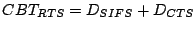
In order to optimize network performance, the Airespace APs are designed to support dynamic channel assignment, client load balancing, and transmission power control. Dynamic channel assignment refers to the technique that switches the AP's operating channel, depending on parameters such as traffic load and the number of users associated with the AP. Client load balancing refers to the technique that controls per-AP user associations. The transmission power control regulates the power at which an AP transmits a frame. Unfortunately, technical details about these three optimizations are proprietary. Nevertheless, we observed that wireless network traffic was fairly well distributed between the three orthogonal channels 1, 6, and 11. Also, the access points were observed to switch channels dynamically to balance the number of users and traffic volume on the three channels.
The method we used to collect data from the MAC layer is called vicinity sniffing [10]. Our vicinity sniffing framework consisted of three sniffers, IBM R32 Think Pad laptops. Each sniffer was equipped with a Netgate 2511 PCMCIA 802.11b radio. The radios were configured to capture packets in a special operating mode called the RFMon mode. The RFMon mode enables the capture of regular data frames as well as IEEE 802.11b management frames. In addition, the RFMon mode records information for each captured packet. This information includes the send rate, the channel used for packet transmission, and the signal-to-noise ratio (SNR) of the received packet. Because the Airespace access points were expected to switch between the 802.11b channels 1, 6, and 11, each sniffer was configured to sniff on one of the three different channels for the duration of each session. The packets were captured using the sniffer utility tethereal. The snap-length of the captured packets was set to 250 bytes in order to capture only the RFMon, MAC, IP and TCP/UDP headers.
The data capturing process was conducted using two different placement configurations, one during the day and the second during the late evening sessions. The late evening sessions are called plenary sessions.
Day sessions: The day sessions were held between 09:00 hrs and 17:30 hrs on March 6-11, 2005. The day sessions were split into 6 to 8 parallel tracks and each track was held in one of the several meeting rooms shown in Figure 2. The parallel session tracks were held at three intervals during the day: 09:00 hrs to 11:30 hrs, 13:00 hrs to 15:00 hrs, and 15:30 hrs to 17:30 hrs. We chose to place the three sniffers in one of the busiest and largest meeting rooms. The placement of the three sniffers is shown in Figure 2. Data was collected during the day sessions held on March 9, 2005.
Figure 2:
Sniffer locations during the day session.
|
Plenary sessions: Plenary sessions were held in a single large meeting room where all the IETF members congregate to discuss administrative issues. The plenary sessions at the IETF were held between 19:30 hrs and 22:30 hrs on March 9 and 10, 2005. Data was collected during the second plenary session held on March 10, 2005. Figure 3 shows the placement of the access points during the plenary session and the single point at which the three sniffers were co-located.
Figure 3:
Sniffer locations during the late evening session.
|
Table 1:
The two sets of IETF wireless network data.
| Data set |
Day |
Ch |
Time |
| 1 |
March 9 2005 |
1 |
11:53-17:30 hrs |
| |
March 9 2005 |
6 |
| |
March 9 2005 |
11 |
| 2 |
March 10 2005 |
1 |
19:30-22:30 hrs |
| |
March 10 2005 |
6 |
| |
March 10 2005 |
11 |
|
Wireless network data collected from the IETF network was separated into two sets named the day session and the plenary session. Table 1 shows the day, time, and channel that each of the two sets represents. Our collection framework recorded a total of 28.6 million data frames, 27.05 million acknowledgment frames, 40,000 RTS frames, and 17,490 CTS frames during the day and the plenary sessions cumulatively. The use of the RTS-CTS mechanism is generally turned off by default on wireless devices and its use is optional. The data indicates that the use of the RTS-CTS mechanism for channel access by conference participants was minimal.
Figure 4:
Data frames, control frames, and number of users statistics.
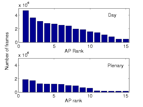 (a) Total number of data and control frames sent and received by the 15 most active APs. Data frames for each AP are represented for the day and plenary sessions.
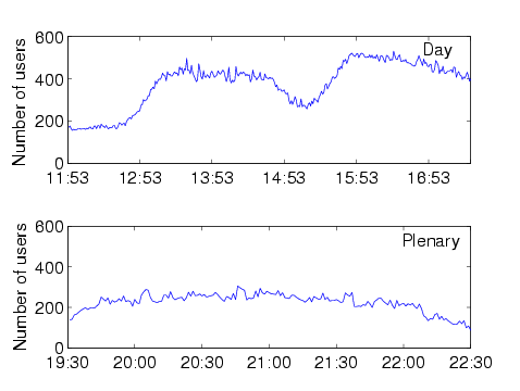 (b) Number of users associated with the wireless network during the day and plenary sessions, averaged over 30 second intervals.
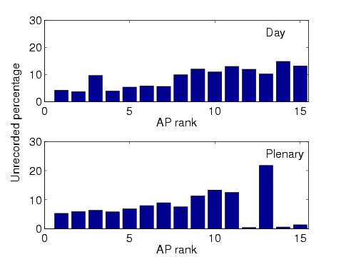 (c) The unrecorded frames percentage computed for the data and control frames sent and received by the 15 most active APs.
|
Per-AP traffic: Figure 4(a) shows the number of data and control frames sent and received by the 15 most active APs out of 152 APs for the day and plenary sessions in decreasing order. We observe that the 15 most active APs during the day session sent and received 90.33% of the total 40.81 million frames, and the 15 most active APs during the plenary session sent and received 95.37% of the total 16.81 million frames.
Number of users: Figure 4(b) shows the instantaneous number of users associated with these access points for the two data sets. For visual clarity, each point on the graph represents the mean number of users in a 30-second interval. We observe that at 15:48 hrs during the day session, a maximum of 523 users were associated with the network, while at 20:45 hrs during the plenary session, a maximum of 325 users were associated with the network. This graph shows that the network was used by a large number of users for almost all of the collection period. In comparison with previous wireless network performance studies, we believe that the number of user associations and the number of frames sent and received by the APs during the day and plenary sessions confirms that the network is large, heavily utilized, and unique in its scale and usage. These traits make the evaluation of the information collected from the network critical and necessary for a clear understanding of heavily utilized and congested networks.
Vicinity sniffing is a technique used to capture control, management, and data frames transmitted by user devices and APs on the wireless portion of the network. In our experiment, we conducted vicinity sniffing using two different sets of sniffer locations for the day and plenary sessions. Vicinity sniffing is the best currently available method to collect link layer information from an operational wireless network. However, the utility of vicinity sniffing is limited by the following factors:
Choice of sniffer locations: The location of one or more sniffers affects the quantity and quality of frames that can be captured from the network. With a priori information about the AP topology and the expected number of frames transmitted to and from the APs, sniffers can be strategically and conveniently placed in the vicinity of those APs. At the IETF, this information was obtained by studying meeting schedules, gathering attendee statistics from meeting organizers, and conducting preliminary activity tests on March 8, 2005. The tests involved the placement of sniffers in different meeting rooms for a short period of time to capture a snapshot of the activity of the APs in the room. These tests allowed us to estimate the behavior of network traffic, number of users, per-AP traffic, and per-channel traffic.
With the information obtained from the preliminary tests and the assumption that users of the wireless network were spread out in different conference rooms, we decided to place three sniffers in three different locations of a single room for the day sessions (shown in Figure 2). This placement allowed us to capture critical data sets from APs and user devices in and around the room. Due to logistical limitations, we co-located the sniffers at a single point during the plenary session, such that a majority of the traffic transmitted by the users and APs in the room could be captured. Since most attendees congregated in the same large room, we assumed that the placement of sniffers at a location in the room would enable us to capture a large portion of the relevant network traffic. The placement of the sniffers during the plenary session is shown in Figure 3.
Unrecorded frames: One of the critical challenges of vicinity sniffing is that the sniffers cannot record all frames that are transmitted over the communication channel. An unrecorded frame belongs to one of three different categories: (1) frames dropped due to bit errors in received frames, (2) hardware limitations that cause dropping of frames during high load conditions [23], and (3) frames that could not be recorded because of the hidden terminal problem.
If the number of unrecorded frames is large, the conclusions drawn from the data set could be inaccurate. Therefore, in this section we discuss the techniques we use to estimate the number of unrecorded control and data frames and the impact of not capturing these frames. The number of unrecorded DATA, RTS, and CTS frames can be estimated using the following techniques.
Data frames: To estimate the number of data frames that were unrecorded by the sniffers, we leverage the DATA-ACK frame arrival atomicity of the IEEE 802.11b DCF standard. The atomicity policy states that if a DATA frame is successfully received by a device in a network, the receiving device should send an ACK after a SIFS delay. No other device in the reception range is allowed to transmit frames during this interval. In other words, when an ACK frame occurs in our traffic logs, we expect a DATA frame to precede it. The source of the DATA frame must be the receiver of the ACK. If this DATA frame is missing, we can assume that our sniffers were unable to capture it.
RTS frames: The use of the RTS-CTS exchange of messages between a source and a destination is optional. However, in our data sets, we detected a limited use of RTS and CTS frames. Consequently, we were able to leverage the RTS-CTS frame arrival atomicity of the IEEE 802.11b DCF standard. It states that if an RTS is successfully received, the receiver may send a CTS after an SIFS delay. No other device in the reception range of the sending device is allowed to transmit frames during this interval. In other words, if a CTS frame is encountered in our data set, we expect an RTS frame to precede it and the receiver of the RTS must be the source of the CTS. If this RTS frame is missing from the data set but the CTS frame was recorded, we can determine that the sniffers were unable to record the RTS.
CTS frames: The number of uncaptured CTS frames can be derived by utilizing the RTS-CTS-DATA frame arrival atomicity of the IEEE 802.11b DCF standard. It states that if RTS and DATA frames are recorded, the receiver of the RTS must have sent a CTS frame following the RTS frame by an SIFS delay. The standard states that the station that sends the RTS will send the following DATA frame only when it receives a CTS from the destination station.
Unfortunately, a drawback of these techniques is that, if both the DATA and ACK frames are missing, or both the RTS and CTS frames are missing, or all three RTS, CTS, and DATA frames are missing, the techniques will fail to determine the DATA, RTS, and CTS frames, respectively, as unrecorded. However, the techniques do provide a close enough estimate of the number of unrecorded frames.
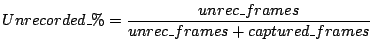
The unrecorded percentage is defined as the percentage of the total frames (control and data frames) that were detected as unrecorded over the sum of the total frames recorded and unrecorded in our data set. We compute the unrecorded percentage using Equation 1 as follows:
 |
(1) |
The unrecorded percentage for each of the 15 most active APs during the day and the plenary sessions is shown in Figure 4(c). The list of APs are ranked in decreasing order of the number of frames sent and received by the APs as shown in Figure 4(a). The figure shows that the unrecorded percentage for the first 15 APs varies between 3% to 15% during the day session, and between 5% to 20% during the plenary session. Based on these values, we assume that the results obtained from the data sets would not be significantly altered even if the occurrence of these frames could be accurately determined. However, to improve the accuracy of the results, we believe that future experiments should use a greater number of sniffers and better hardware to reduce the number of unrecorded frames caused by hidden terminals and hardware limitations.
Defining Congestion
On the Internet, a network link is said to be congested when the offered load on the link reaches a value close to the capacity of the link. In other words, we can define congestion as the state in which a network link is close to being completely utilized by the transmission of bytes. In a similar manner, wireless network congestion can be defined as the state in which the transmission channel is close to being completely utilized. The extent of utilization can be measured using a channel busy-time metric given as the fraction of a set period of time that a channel is busy.
In this section, we show how channel utilization is used in conjunction with the computed throughput and goodput of the channel to estimate a set of utilization thresholds to identify levels of congestion in the network. We also show that the effects of congestion on link layer behavior can be better explained by defining levels of congestion as compared to exact values of utilization.
Channel utilization for a set period of time is computed on a percentage scale. In our study, we choose to use one second as the period. We find that this interval is an appropriate granularity in our analysis.
The utilization of a network channel per second is computed by adding (1) the time utilized by the transmission of all data, management, and control frames recorded by our sniffers, and (2) the total number of delay components such as the Distributed Inter-frame Spacing (DIFS) and Short Inter-frame Spacing (SIFS) during the same second. These delays form a part of the channel utilization computation because, during this period, the medium remains unshared between the stations in the network. The communication channel is unshared when no other station in the vicinity of the station that holds the channel can transmit frames for the specified delay time. In this paper we use delay component values suggested by Jun et al. [11]. Table 2 shows the delay in microseconds for delay components of the IEEE 802.11b protocol.
As previously described, Figure 1 shows the timing diagram for the CSMA/CA and (RTS/CTS) mechanisms. The diagram suggests a specific ordering of delay components. For instance, a DATA packet is preceded by SIFS delays, an RTS packet is preceded by a DIFS delay, and an ACK packet is preceded by an SIFS delay. In the heavily utilized IETF network where hundreds of users are associated with the network simultaneously, at any given instant, a minimum of a single user is ready to send a packet. In other words, we assume that at least one station has a BO timer equal to zero, at any instant. Therefore, the average time spent in the Back-off (BO) state will be equal to zero, i.e.,  = 0. = 0.
The delay components specified in Table 2 suggest that, first, the channel utilization increases for larger data frames since a larger number of bytes take greater time to transmit. Second, channel utilization increases with a decrease in the rate at which data frames are transmitted.
And third, the data frame Physical Layer Convergence Protocol (PLCP) header is always transmitted with a fixed delay equal to  . .
Table 2:
Delay components specified in microseconds.
|
Delay Component |
Delay ( sec.) sec.) |
 |
50 |
 |
10 |
 |
352 |
 |
304 |
 |
304 |
 |
304 |
|
|
0 |
|
|
192 |
 |
 ) ) |
|
To accurately compute the channel utilization for a packet encountered in our data set, we use the timing diagram shown in Figure 1 and the delay component values in Table 2. Depending on the type of control frame and the rate and size of a data frame, the channel busy-time for the frame is computed as follows:
Data frames: A DIFS interval occurs before each data frame, either immediately before the data frame, in the case when the RTS-CTS mechanism is not utilized, or before the RTS frame, in the case when RTS-CTS is used. The DIFS delay interval is used for the busy-time computation of a data frame. The channel busy-time (CBT) for a data frame of size, S bytes, sent at a rate R, is computed using Equation 2.
 |
(2) |
RTS frames: In the case when RTS frames are encountered in our data set, the CBT for the frames is computed using Equation 3.
 |
(3) |
CTS frames: When a CTS frame is encountered in our data set, Figure 1 suggests that the CTS frame is transmitted following an SIFS delay after the RTS frame was received. Hence, the CBT for CTS frames is computed using Equation 4.
 |
(4) |
ACK frames: When an ACK frame is encountered in our data set, Figure 1 suggests that the ACK frame is transmitted following an SIFS delay after the preceding data frame was received. Hence, the CBT for ACK frames is computed using Equation 5.
 |
(5) |
Figure 5:
Utilization percentage and frequency distribution.
 (a) Percentage utilization for the day session.
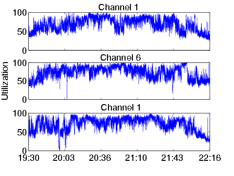 (b) Percentage utilization for the plenary session.
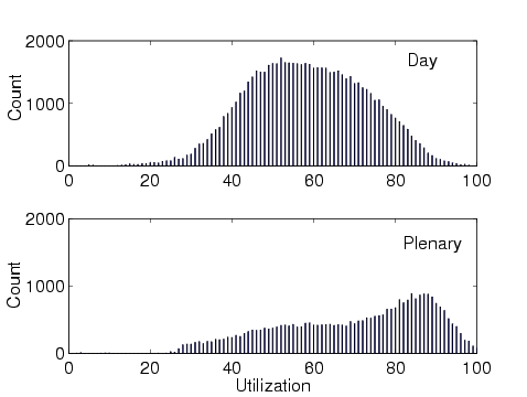 (c) Frequency of percentage utilization values.
|
Beacon frames: A beacon frame is typically sent by each AP in the network at 100 millisecond intervals. The beacon frames are preceded by a DIFS delay interval. Hence, when a beacon frame is encountered in the data set, the CBT is computed using Equation 6.
 |
(6) |
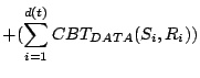
The CBT of the channel for a one second interval, t, is the total delay computed for all data and control frames that are transmitted within a second. Therefore, if r(t) RTS frames, c(t) CTS frames, a(t) ACK frames, b(t) beacon frames, and d(t) data frames are encountered during the same one second interval, the total CBT for the interval is calculated using Equation 7.
The percentage channel utilization over the one second interval,  , is computed using Equation 8 as follows: , is computed using Equation 8 as follows:
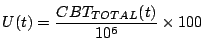 |
(8) |
Equation 8 is used to compute the percentage utilization of the channel per second during the day and the plenary sessions.
Utilization frequency: The utilization computations are graphed on a time-series plot in Figure 5(a) for the day session and Figure 5(b) for the plenary session. Figure 5(c) is a histogram that shows the frequency of percentage utilization for the day and plenary sessions; for instance, the channel was 53% utilized for 1823 seconds during the day session. The histograms indicate that during the day the channel most often experienced about 55% utilization, while during the plenary, the channel was most often utilized at about 86%. During the day session, users were distributed across all the meeting rooms, and hence, fewer data and control frame transmissions were collected by the sniffers. On the other hand, users congregated closer to the sniffers during the plenary session, and hence, a larger number of transmissions can be collected by the sniffers. The proximity of users to the sniffers thus results in a higher channel utilization levels.
Figure 5(c) shows that there is not a significant period of time when the network was 0-30% or 99-100% utilized and so it is difficult to use our data set to characterize the behavior of the network. Thus, the evaluation of link-layer behavior in this paper focuses on the periods when the network was utilized between 30-99%.
Figure 6:
Channel throughput and goodput per second calculated at the corresponding channel utilization.
|
The throughput of the channel for a one second interval is the sum of the total number of bits of all recorded frames transmitted over the wireless channel during a one second interval. The goodput of the channel is the total number of recorded bits of all the control and successfully acknowledged data frames transmitted over the wireless channel during a one second interval.
Figure 6 shows the throughput and goodput of the channel versus channel utilization. Each point value y in the figure represents the average throughput or goodput over all one second intervals during the day and plenary sessions that are x% utilized. The number of one second intervals is equal to the frequency of percentage utilization of the channel shown in Figure 5(c). Figure 6 indicates that as the channel utilization increases from 30% to 84%, the average throughput of the channel increases to 4.9 Mbps and the average goodput increases to 4.4 Mbps. The average throughput at 84% channel utilization is closest to the achievable theoretical maximum throughput [11]. Since the computation of throughput includes all the transmitted frames, the calculated throughput value for each utilization percentage is higher than the corresponding value of goodput.
For channel utilization between 84% and 98%, we observe a significant decrease in throughput, from 4.9 Mbps to 2.8 Mbps, and a decrease in goodput, from 4.4 Mbps to 2.6 Mbps. This decrease in the throughput and goodput with a concomitant increase in channel utilization of the wireless network is due to the multirate adaptation algorithms. As channel utilization increases, a large number of frame errors and retransmissions occur. As retransmissions increase, most network cards decrease the rate at which each data packet is transmitted. At lower data rates (i.e., 1 Mbps), frames occupy the channel for a longer period of time, and hence, fewer bytes are transmitted over the channel. Heusse et al. state that the use of lower data rates for data frames penalizes the delivery of data frames transmitted at higher rates and is an anomaly of the IEEE 802.11 DCF protocol [8]. Therefore, we believe that at channel utilization levels greater than 84%, the transmission of data frames at the lower data rates of 1 or 2 Mbps significantly reduces the throughput of the network. Section 6 presents results that confirm this hypothesis.
From our observations, we believe that the wireless communication channel is highly congested when the throughput and goodput of the wireless channel decreases after reaching their respective maximums.
For the wireless network at the IETF, we define the network to be highly congested when the channel utilization level is greater than 84%. In this paper we also use the saturation throughput and goodput observations to classify congestion in the communication channel. The variations in link layer behavior, such as the effectiveness of the RTS-CTS mechanism, the number of successfully acknowledged data frames, retransmissions, and the acceptance delay of data frames can be better explained by using congestion classes, as described in the next section.
In this paper, we suggest that congestion in an IEEE 802.11b wireless network can be classified by using the observed trends in throughput and goodput with respect to increasing channel utilization levels. We classify network states into three classes: uncongested, moderately congested, and highly congested. In the case of the IETF wireless network, an uncongested channel is a channel that experiences less than 30% utilization. Since the throughput and goodput of the channel shows a gradual increase from 30% utilization to 84%, the channel is moderately congested for utilization values in the range of the 30%-84%. A channel is stated to be highly congested when the channel utilization is greater than the 84% threshold.
Effects of Congestion
This section discusses the effect of the different congestion levels on network characteristics, behavior of the RTS-CTS mechanism, channel busy-time, reception of frames of different sizes transmitted at different rates, and acceptance delays for data packets. These characteristics offer a basis for understanding the operation of the IEEE 802.11b MAC protocol in heavily congested networks.
To better understand the effects of congestion, we categorize a frame into one of 16 different categories. The categories are defined as a combination of (1) the four possible data rates: 1, 2, 5.5, and 11 Mbps, and (2) the four different frame size classes: small, medium, large and extra-large. The frames are split into the four size classes so that the effect of congestion on different sized frames can be derived separately. The four size classes are defined as follows:
Small (S): frame sizes between 1-400 bytes
Medium (M): frame sizes between 401-800 bytes
Large (L): frame sizes between 801-1200 bytes
Extra-large (XL): frame sizes greater than 1200 bytes
The behavior of the small size class is representative of short control frames and data frames generated by voice and audio applications. The medium, large, and extra-large size class represents the frames generated by file transfer applications, SSH, HTTP, and multimedia video applications.
Figure 7:
Average number of RTS and CTS frames transmitted per second on the wireless channel versus the channel utilization.
|
The RTS-CTS mechanism helps reduce frame collisions due to hidden terminals. However, the use of the mechanism is optional. In our data sets we observe that only a small fraction of data frames utilized the RTS-CTS frames to access the channel for transmission. Figure 7 shows that as channel utilization increased, the number of RTS frames increased. Specifically, in the moderate congestion range between 80% and 84% utilization, the average number of RTS frames transmitted per second shows an increase from 5 to 8. This is because, as utilization increases, a greater number of collisions results in a greater number of RTS frames required to access the medium. At the same time, the number of CTS frames does not increase at the same rate because of the failure to receive the RTS frames.
At high congestion levels, the number of RTS frames decreases rapidly because congestion in the medium limits channel access opportunities for their transmission. The number of CTS frames also decreases at high congestion levels because receivers experience a similar limitation for channel access.
When a limited number of devices use the RTS-CTS mechanism, fair channel access for the devices that use the mechanism is also limited. That is because, the devices that utilize the mechanism to transmit DATA frames rely on the successful delivery of the RTS and CTS frames preceding the DATA frame. On the other hand, devices that do not utilize the mechanism solely rely on the successful delivery of the DATA frame. During congestion, this problem is more pronounced because the probability of the delivery of frames decreases due to collisions. Thus, our observations suggest that the use of the RTS-CTS mechanism is deemed to be unfair in congested networks in which only a small set of users depend on the mechanism.
Figure 8:
Channel busy-time share of each of the four data rates versus the channel utilization.
|
Figure 9:
Average number of bytes transmitted per second at each of the four data rates versus the channel utilization.
|
Channel busy-time is defined as the fraction of the one second interval during which the channel is either occupied by the transmission of frame bytes or IEEE 802.11b standard specified delays between frame transmissions. In this section, we evaluate the effect of different levels of congestion on the channel busy-time measure for the four different data rates. In Section 5 we observed that, during high congestion, the network throughput and goodput decrease as channel utilization increases. The drop in throughput and goodput can be attributed to the large number of low data rate frames transmitted on the channel. This observation can be better understood by using the trends illustrated in Figure 8.
Figure 8 shows the fraction of a one second interval occupied by 1, 2, 5.5, and 11 Mbps frames at each channel utilization level. Figure 9 shows the total number of bytes transmitted on the channel per second at each channel utilization level. The figures suggests that the average fraction of a one second period occupied by the 1 Mbps frames is much greater than the time occupied by the frames transmitted at 11 Mbps, even though the number of bytes transmitted at 11 Mbps is significantly greater than the number of bytes transmitted at 1 Mbps at almost all levels of channel utilization. Moreover, during high congestion, the average fraction of one second occupied by 1 Mbps frames increases from 0.43 seconds to 0.54 seconds. As the fraction occupied by the transmission of 1 Mbps frames increases, the throughput and goodput of the network decrease. This confirms our hypothesis that the drop in the throughput and goodput during high congestion is because of the larger fraction of time occupied by slower 1 Mbps frames in the network.
Figure 10:
Average number of small data frames transmitted per second on the wireless channel versus the channel utilization.
|
Figure 11:
Average number of extra-large data frames transmitted per second on the wireless channel versus the channel utilization.
|
Figure 12:
Average number of data frames transmitted per second at 1 Mbps data rate on the wireless channel versus the channel utilization.
|
Figure 13:
Average number of data frames transmitted per second at 11 Mbps data rate on the wireless channel versus the channel utilization.
|
In this section we provide statistics on the number of data frames transmitted on the channel at the four data rates (1, 2, 5.5, and 11 Mbps) and for each frame size class (S, M, L, and XL). The naming convention for the type of frames follows a size-rate format. For instance, an S frame transmitted at 11 Mbps is named S-11 and an XL frame transmitted at 1 Mbps is named XL-1.
Figure 10 shows the average number of frames of size S transmitted per second on the channel at each channel utilization. Each point on the graph is an average over our entire data set, including both the day and the plenary session. The number of frames transmitted per second includes both the frames sent at the first attempt and retransmitted frames. We observe that as utilization increases, the number of transmitted S-1, S-2, S-5.5, and S-11 frames increases. However, the number of S-11 frames is significantly larger than the number of frames sent at the other data rates. Cantieni et al. present analytical results that suggest that when an IEEE 802.11b wireless network experiences a state of congestion or throughput saturation, the smaller sized frames sent at the highest rate of 11 Mbps have a higher probability of successful transmission [4] that frames sent at lower rates. In line with these results, we observe a rise in the number of S-11 frames transmitted during high congestion.
Figure 11 shows the average number of XL frames transmitted per second on the channel at each utilization level. We observe that the number of XL-11 frames is greater than the number of frames sent at lower rates. During congestion, the number of XL-11 frames transmitted per second also increases. This increase can be attributed to the increase in the channel access capability of 11 Mbps frames.
Figure 12 shows the average number of frames transmitted at 1 Mbps per second at each channel utilization level. The figure shows that there were a greater number of S-1 frames in the data set compared to the number of XL-1 frames transmitted per second. During high congestion we observe that the number of S-1 and XL-1 frames showed an increase. The increase can be attributed to the multirate adaptation algorithms that decrease the sending rate for frame retransmissions.
Figure 13 shows the average number of frames transmitted at 11 Mbps per second at each channel utilization level. The figure indicates that a large number of data frames are transmitted at the highest data rate. However, during high congestion the number of S-11 and XL-11 frames transmitted per second increases as channel utilization increases. This increase can be attributed to the increase in the number of retransmissions during high congestion.
Figure 14:
Average number of data frames successfully acknowledged per second at their first attempt of transmission versus the channel utilization.
|
In this section we evaluate the number of successfully acknowledged data frames that were acknowledged at their first attempt of transmission. The evaluation of frame reception includes statistics for S-1, XL-1, S-11 and XL-11 frames. We believe that the evaluation of the behavior of this set of frames is representative of the whole set of results.
A successfully acknowledged data frame is defined as a data frame for which the source receives an acknowledgment frame from the receiving station within an SIFS time delay. In our data set, we identify acknowledged frames as data frames that are immediately followed by an acknowledgment from the receiving station. Other cases include: (1) when the receiving station does not send an acknowledgment because it failed to receive the data frame successfully, (2) the receiving station sends an acknowledgment but the sniffer failed to capture the frame due to either bit errors or the hidden terminal problem, or (3) when the acknowledgment frame from the receiving station was not encountered immediately following the data frame sent by the sending station; the frame is considered to be not acknowledged or dropped.
Figure 14 shows the average number of data frames per second that were acknowledged at their first attempt at transmission for different channel utilization levels. The figure shows that during moderate congestion, there is an increase in the number of 11 Mbps frames acknowledged per second. But, at utilization levels specifically between 80% and 84%, the number of 11 Mbps frames acknowledged per second decreases due to contention in the network. However, during high congestion, the number of 11 Mbps frames that are successfully acknowledged increases. The increase can be attributed to the higher probability of the faster 11 Mbps frames being received as the number of slow 1 Mbps frames transmitted in the network increases.
Thus, our conclusion from this observation is that the reduced sending rate causes a decrease in the throughput achieved during congestion due to larger CBTs of 1 Mbps frames. Also, 11 Mbps frames have a higher probability of reception during high congestion.
Figure 15:
Acceptance delay (in seconds) for data frames successfully acknowledged per second versus the channel utilization.
|
The Acceptance Delay for a data frame is the time taken for a data frame to be acknowledged, independent of the number of attempts to transmit. In other words, it is the time computed between the transmission of a data frame and the time when the acknowledgment was recorded. Evaluation of the acceptance delay is significant because it gives us an opportunity to observe the average time taken for a data frame to be delivered and acknowledged at increasing channel utilization levels. Our hypothesis is that the acceptance delay information at different channel utilization levels can be used to make intelligent decisions about choosing data send-rates.
Figure 15 shows the acceptance delays computed for S-1, S-11, XL-1, and XL-11 frames that were successfully acknowledged during the day and the plenary sessions. We observe a noticeable rise in the acceptance delays as utilization levels increase. However, the acceptance delay values for S-1 and XL-1 frames are significantly greater than the acceptance delays for S-11 and XL-11 frames. The figure also shows that the acceptance delays for S-1 frames are greater than the acceptance delays for XL-11 frames. This observation indicates that the performance of frames that are transmitted at 11 Mbps is better than the performance of frames sent at 1 Mbps, independent of the size of the frames. Additionally, the figure shows that acceptance delays for XL-1 frames are greater than the acceptance delays for S-1 frames. On the other hand, S-11 and XL-11 frames exhibit very similar acceptance delay curves. Therefore, we conclude that the size of a frames transmitted at 1 Mbps has a significant effect on the acceptance delays.
In summary, we hypothesize that for better upper layer protocol performance and to maintain overall network throughput, transmitting data frames at higher rates is better than transmitting frames at lower rates.
Conclusions
The analysis of heavily congested wireless networks is crucial for the robust operation of such networks. To this end, this paper has presented an analysis of a large-scale IEEE 802.11b wireless network deployed at the Internet Engineering Task Force meeting in Minneapolis, Minnesota. Specifically, we have investigated the effect of congestion on network throughput and goodput, channel busy-time, the RTS-CTS mechanism, frame transmission and reception, and acceptance delay. However, we believe that the data sets that we collected through vicinity sniffing techniques can be further analyzed to further broaden our scope of understanding.
Observations made in this paper suggest that the use of lower data rates to transmit frames in the network significantly decreases the network throughput and goodput. Therefore, the use of low data rates between two nodes should only be used to alleviate frame losses occurring due to bit errors, low signal-to-noise (SNR) ratio of received frames, or the transmission of frames to greater distances. During congestion, higher data rates should be used. However, the multirate adaptation scheme implemented in commodity radios does not distinguish between frame losses that occur due to any of these causes. Consequently, the response of multirate adaptation schemes to frames losses often results in the poor choice of transmission rates in heavily congested environments. As a result, overall network performance is adversely impacted. Alternate multirate adaptation schemes [9,18] that determine an optimal packet transmission rate based on SNR may offer some relief. As another strategy to utilize high data rates, clients may choose to dynamically increase or decrease the transmit power of the radio such that data frames can be consistently and reliably transmitted at high data rates.
Another observation made in the paper is the failure of the RTS-CTS mechanism to provide fair channel access to the few nodes using the mechanism. Therefore, during high congestion, the use of the mechanism should be avoided.
Funding for this work is in part through NSF Network Research Testbeds (NRT) grant ANI-0335302 as part of the WHYNET project and a grant from Nokia Research through the UC Micro program. We would like to thank Jim Martin (Netzwert AG), Karen O Donoghue (Naval Surface Warfare Center), Bill Jensen (University of Wisconsin), Jesse Lindeman (Airespace), and the IETF62 NOC Team for assisting us in the collection of the data used in this paper.
- 1
-
I. Aad, Q. Ni, C. Barakat, and T. Turletti.
Enhancing IEEE 802.11 MAC in Congested Environments.
In Proceedings of IEEE ASWN, Boston, MA, August 2004.
- 2
-
A. Balachandran, G. M. Voelker, P. Bahl, and P. V. Rangan.
Characterizing User Behavior and Network Performance in a Public
Wireless LAN.
In Proceedings of ACM SIGMETRICS, pages 195-205, Marina Del
Rey, CA, June 2002.
- 3
-
M. Balazinska and P. Castro.
Characterizing Mobility and Network Usage in a Corporate Wireless
Local-area Network.
In Proceedings of ACM MOBICOM, San Francisco, CA, May 2003.
- 4
-
G. R. Cantieni, Q. Ni, C. Barakat, and T. Turletti.
Performance Analysis under Finite Load and Improvements for
Multirate 802.11.
Elsevier Computer Communications Journal, 28(10):1095-1109,
June 2005.
- 5
-
S. Cen, P. C. Cosman, and G. M. Voelker.
End-to-end Differentiation of Congestion and Wireless Losses.
ACM/IEEE Transactions on Networking, 11(5):703-717, October
2003.
- 6
-
F. Chinchilla, M. Lindsey, and M. Papadopouli.
Analysis of Wireless Information Locality and Association Patterns
in a Campus.
In Proceedings of IEEE INFOCOM, Hong Kong, March 2004.
- 7
-
T. Henderson, D. Kotz, and I. Abyzov.
The Changing Use of a Mature Campus-wide Wireless Network.
In Proceedings of ACM MOBICOM, Philadelphia, PA, September
2004.
- 8
-
M. Heusse, F. Rousseau, G. Berger-Sabbatel, and A. Duda.
Performance Anomaly of 802.11b.
In Proceedings of IEEE INFOCOM, San Francisco, CA, March-April
2003.
- 9
-
G. Holland, N. Vaidya, and P. Bahl.
A Rate-Adaptive MAC Protocol for Multi-Hop Wireless Networks.
In Proceedings of ACM MOBICOM, pages 236-251, Rome, Italy,
July 2001.
- 10
-
A. Jardosh, K. Ramachandran, K. Almeroth, and E. Belding-Royer.
Understanding Link-Layer Behavior in Highly Congested IEEE 802.11b
Wireless Networks.
In Proceedings of ACM SIGCOMM Workshop E-WIND, Philadelphia,
PA, August 2005.
- 11
-
J. Jun, P. Peddabachagari, and M. Sichitiu.
Theoretical Maximum Throughput of IEEE 802.11 and its Applications.
In Proceedings of the IEEE International Symposium on Network
Computing and Applications, pages 249-257, Cambridge, MA, April 2003.
- 12
-
A. Kamerman and L. Monteban.
WaveLAN 2: A High-performance Wireless LAN for the Unlicensed Band.
In Bell Labs Technical Journal, Summer 1997.
- 13
-
D. Kotz and K. Essien.
Analysis of a Campus-wide Wireless Network.
In Proceedings of ACM MOBICOM, Atlanta, GA, September 2002.
- 14
-
X. Meng, S. Wong, Y. Yuan, and S. Lu.
Characterizing Flows in Large Wireless Data Networks.
In Proceedings of ACM MOBICOM, Philadelphia, PA, September
2004.
- 15
-
A. Mishra, M. Shin, and W. A. Arbaugh.
An Empirical Analysis of the IEEE 802.11 MAC Layer Handoff Process.
ACM SIGCOMM Computer Communication Review, 33(2):93-102, 2003.
- 16
-
E. Modiano.
An Adaptive Algorithm for Optimizing the Packet Size Used in
Wireless ARQ Protocols.
Wireless Networks, 5(4):279-286, July 1999.
- 17
-
M. Rodrig, C. Reis, R. Mahajan, D. Wetherall, and J. Zahorjan.
Measurement-based Characterization of 802.11 in a Hotspot Setting.
In Proceedings of EWIND, Philadelphia, PA, August 2005.
- 18
-
B. Sadeghi, V. Kanodia, A. Sabharwal, and E. Knightly.
Opportunistic Media Access for Multirate Ad Hoc Networks.
In Proceedings of ACM MOBICOM, pages 24-35, Atlanta, USA,
September 2002.
- 19
-
D. Schwab and R. Bunt.
Characterizing the Use of a Campus Wireless Network.
In Proceedings of IEEE INFOCOM, Hong Kong, March 2004.
- 20
-
Y. Tay and K. Chua.
A Capacity Analysis for the IEEE 802.11 MAC Protocol.
Wireless Networks, 7(2):159-171, March 2001.
- 21
-
M. Torrent-Morenoe, D. Jiang, and H. Hartenstein.
Broadcast Reception Rates and Effects of Priority Access in 802.11
Based Vehicular Ad hoc Networks.
In Proceedings of ACM VANET, Philadelphia, PA, October 2001.
- 22
-
C. Tuduce and T. Gross.
A Mobility Model Based on WLAN Traces and its Validation.
In Proceedings of IEEE INFOCOM, Miami, FL, March 2005.
- 23
-
J. Yeo, M. Youssef, and A. Agrawala.
A Framework for Wireless LAN Monitoring and its Applications.
In Proceedings of the ACM Workshop on Wireless Security, pages
70-79, Philadelphia, PA, October 2004.
Understanding Congestion in IEEE 802.11b Wireless Networks
This document was generated using the
LaTeX2HTML translator Version 2002-2 (1.70)
Copyright © 1993, 1994, 1995, 1996,
Nikos Drakos,
Computer Based Learning Unit, University of Leeds.
Copyright © 1997, 1998, 1999,
Ross Moore,
Mathematics Department, Macquarie University, Sydney.
The command line arguments were:
latex2html -split 0 imc.tex
The translation was initiated by Amit Jardosh on 2005-11-17


Amit Jardosh
2005-11-17
|