Dividing the CPUs of an SMP into pools for scheduling decisions, has the welcome effect of improving the scalability of the scheduling algorithms. However, this kind of limiting introduces the problem of load imbalance between the CPUs in different pools. We focus on two kinds of imbalances depending on what is defined as the load :
The load imbalances mentioned here only pertain to non-real time (SCHED_OTHER) tasks as MQS and PMQS maintain real time tasks on a separate global runqueue.
The existence of load imbalances does not necessarily call for corrective measures. For high end systems where system throughput is generally more important than job response times, isolating CPU pools from each other might be desirable. In such cases, priority inversion is not an issue and it is sufficient to ensure that all CPUs have enough tasks and that the initial placement of tasks (amongst pools) is balanced.
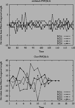
In this paper we examine various load balancing mechanisms under PMQS and compare their efficacy and their overall performance impact on various workloads as compared to DSS and MQS. These mechanisms are LBOFF, IP, LBC and LBP and are described below. To establish their efficacy we use the two distinct workloads, namely Mkbench and Chat, to monitor runqueue length per CPU for a 4-way SMP system. PMQS is configured with a poolsize of 1. We show for these benchmarks and configurations the deviation from the mean runqueue length at one second intervals. Mkbench was run with 2 simultaneous kernel builds with ``-j 16'' yielding an average load of 32 or 8 per CPU. Chat was run with 10 rooms and 900 messages, which yielded an average of 207 runnable tasks or 52 per run queue.
Figure 1 shows the load imbalances that are achieved under Mkbench and Chat when running PMQS with poolsize=4, which is basically equivalent to MQS. For Mkbench the individual runqueue length of the various CPUs falls into a narrow range of
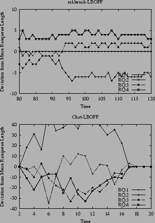
LBOFF simply utilizes CPU pooling without any attempt to balance load among the pools or CPUs. With poolsize=1, the runqueues are isolated from each other. The only means for a process to migrate from one CPU to another is during reschedule_idle() invocations when there exist idle processors on remote pools. Figure 2 shows the load imbalances that are achieved under Mkbench and Chat. For both, the per-CPU load can deviate quite substantially. We use this graph as a reference point for evaluating the load balancers below.
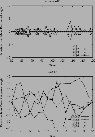
In initial placement (IP), a task is moved to the least loaded CPU as defined by the CPU's runqueue length, when a new program is launched, i.e. at sys_execv() time. Figure 3 shows that IP is very effective in equalizing the runqueue lengths in an environment of short lived processes. On the other hand, in environments with long lived processes IP is ineffective.
We compare this static approach to the problem of load imbalance with a flexible and dynamic load balancing mechanism. This flexible mechanism allows a system administrator to choose between the extremes of isolating CPUs (LBOFF) and treating them as one entity for scheduling (as is done by MQS). To do this, we provide an external load balancer module (LB) which balances the runqueues of CPUs belonging to different pools based on user-specified parameters and and a load function determining the CPU-load weight of each runqueue towards the overall load. So far we have considered two load functions. The runqueue_length load function is simply the length of the CPU runqueue and the runqueue_na_goodness load function is computed by summing the non-affinity goodness values of each task on a runqueue. The results presented in this paper are based on the runqueue_length function.
The LB module is invoked periodically through a timer function. The frequency of invocation is controlled through a user-specified parameter which can be dynamically altered through a /proc interface. Unless otherwise noted, the LB is invoked every 600 milliseconds. On each invocation, LB first records the load on each CPU runqueue. Once individual runqueue loads have been determined, LB computes the average load across the system. Runqueues are marked as having a ``surplus'' or ``deficit'' load.
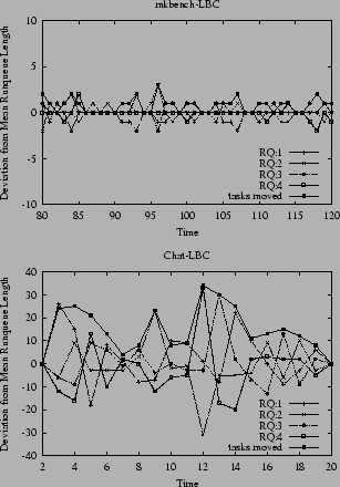
From here we have experimented with two different version of load balancers, called LBC and LBP. LBC (Load Balancing across all Cpus), tries to equalize all runqueues within the system tightly. For that LBC first performs intra-pool balancing by transferring tasks from surplus to deficit runqueues within each pool until runqueue loads are equal the average. In the second stage, tasks are transferred between the remaining surplus to deficit runqueues system wide, reflecting an inter-pool balancing. In the following figures we also plot the total number of tasks moved during the LB phase to indicate the corrective actions taken by the LB after the observed state. Figure 4 shows that for Mkbench, LBC controls the runqueue length very tightly and needs to typically move only one or two tasks. For Chat, however, Figure 4 shows that LBC's tight balancing act leads to over correction as is clearly seen in states t=5,13,14. The statistics are summarized in Table 1. For LBC an average of 11.5% of tasks are moved every LB invocation with a maximum of 23.1%.
We, therefore, developed LBP (Load Balancing across all Pools), which differs from LBC in two aspects. First, it does not perform any intra-pool balancing on the assumption that schedule() and reschedule_idle() do a good enough job of load balancing within a pool as shown in Figure 1. Second, it defines a user-specified error tolerance factor to avoid over aggressive corrections leading to the oscillation seen in Figure 4. A runqueue is considered balanced, if its load is within the error tolerance of the system average load. Tasks from surplus queues are transferred to deficit queues only if they are in distinct pools. The error tolerance factor is dynamically configurable through the /proc interface. Since poolsize=1 was selected for this evaluation, the following figures simply demonstrate the effects of the error tolerance.
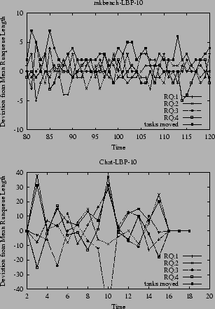
Figure 5 shows the profile for LBP-10, i.e. LBP with a error tolerance of 10%. Combined with the statistics in Table 1, we observe that average number of tasks moved has been reduced to 5.6%. The combined average runqueue length is 179, which amounts to 45 per CPU. Only if the individual runqueue length differs more than 5 from the mean does LBP-10 try to balance that queue. The oscillations observed under LBC are significantly reduced.
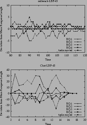
Figure 6 shows the profile for LBP-45, i.e. LBP with a error tolerance of 45%. Combined with the statistics in Table 1, we observe that average number of tasks moved has been reduced to 0.9%. The combined average runqueue length is 178, which amounts to 45 per CPU. Only if the individual runqueue length differs more than 20 from the mean does LBP-45 try to balance that queue. The oscillations observed under LBC and LBP-10 are virtually eliminated.
For Mkbench, Figure 5 actually shows worse oscillating behavior for LBP-10 as compared to LBC, requiring more aggressive task movements. In contrast, LBP-45 initiates a significantly smaller number of task moves, resulting in a smoother profile. However neither LBP is capable too obtain the close balanced achieved in IP and LBC.
To summarize, in this section we introduced various load balancing mechanisms. We observed that these mechanisms in general are effective in balancing the lengths of the individual runqueues. However, we also observed that the runqueue length are sensitive to the nature of the workload and that tight load balancing methods can have adverse effects. In the next section, we will evaluate the overall performance effects of load balancing techniques.